Statistical Genomics Lecture 18 SUPER Zhiwu Zhang Washington

Statistical Genomics Lecture 18: SUPER Zhiwu Zhang Washington State University

Outline • Kinship based on QTN • Confounding between QTN and kinship • Complimentary kinship • SUPER

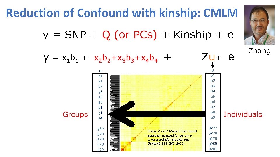
Reduction of Confound with kinship: CMLM y = SNP + Q (or PCs) + Kinship + e y = x 1 b 1 + x 2 b 2+x 3 b 3+x 4 b 4 + Zu+ e Zhang Individuals Groups Zhang, Z. et al. Mixed linear model approach adapted for genomewide association studies. Nat Genet 42, 355– 360 (2010).

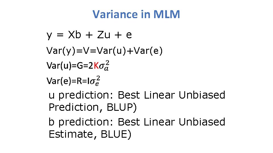
Variance in MLM y = Xb + Zu + e Var(y)=V=Var(u)+Var(e) u prediction: Best Linear Unbiased Prediction, BLUP) b prediction: Best Linear Unbiased Estimate, BLUE)

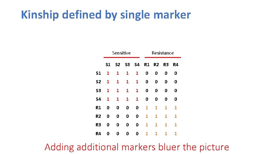
Kinship defined by single marker Sensitive Resistance S 1 S 2 S 3 S 4 R 1 R 2 R 3 R 4 S 1 1 1 0 0 S 2 1 1 0 0 S 3 1 1 0 0 S 4 1 1 0 0 R 1 0 0 1 1 R 2 0 0 1 1 R 3 0 0 1 1 R 4 0 0 1 1 Adding additional markers bluer the picture

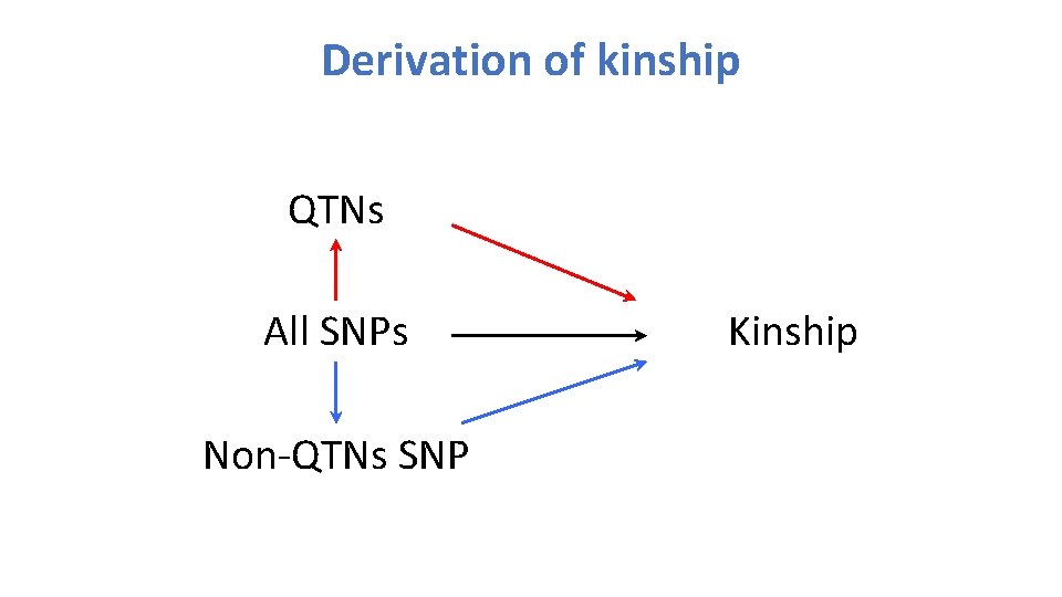
Derivation of kinship QTNs All SNPs Non-QTNs SNP Kinship

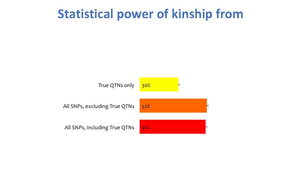
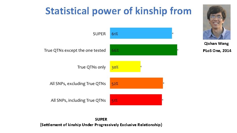
Statistical power of kinship from

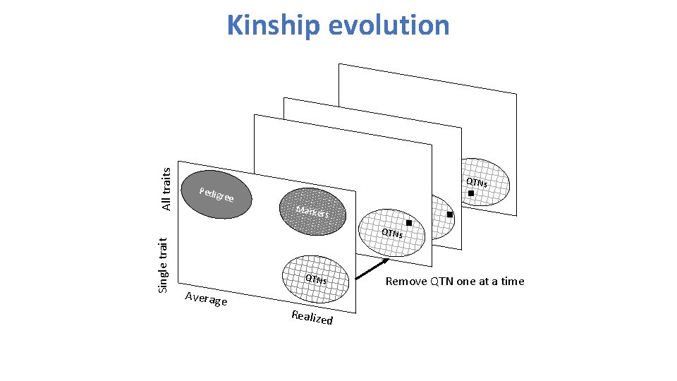
Single trait All traits Kinship evolution QTNs Pedig ree Marke rs QTNs Average Realize Remove QTN one at a time d

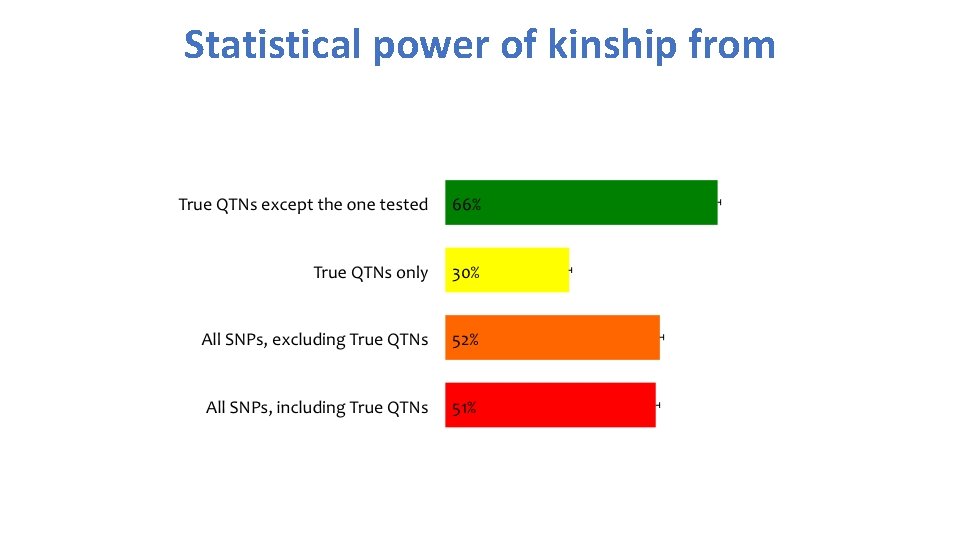
Statistical power of kinship from

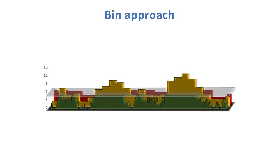
Bin approach

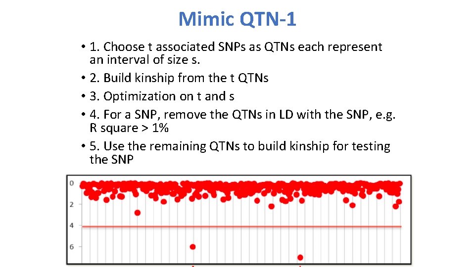
Mimic QTN-1 • 1. Choose t associated SNPs as QTNs each represent an interval of size s. • 2. Build kinship from the t QTNs • 3. Optimization on t and s • 4. For a SNP, remove the QTNs in LD with the SNP, e. g. R square > 1% • 5. Use the remaining QTNs to build kinship for testing the SNP

Statistical power of kinship from Qishan Wang PLo. S One, 2014 SUPER (Settlement of kinship Under Progressively Exclusive Relationship)

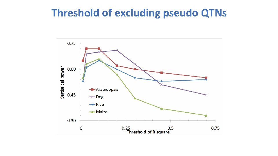
Threshold of excluding pseudo QTNs

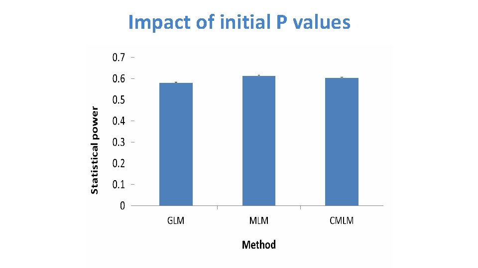
Impact of initial P values

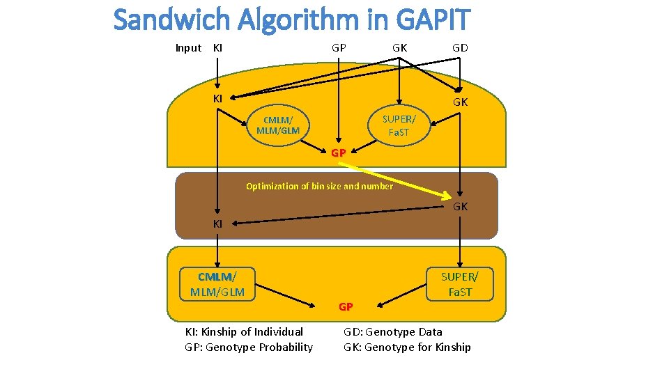
Sandwich Algorithm in GAPIT Input KI GP GK KI GD GK SUPER/ Fa. ST CMLM/GLM GP Optimization of bin size and number GK KI CMLM/ CMLM MLM/GLM KI: Kinship of Individual GP: Genotype Probability GP SUPER/ Fa. ST GD: Genotype Data GK: Genotype for Kinship

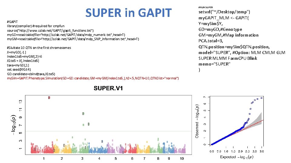
SUPER in GAPIT #GAPIT library(compiler) #required for cmpfun source("http: //www. zzlab. net/GAPIT/gapit_functions. txt") my. GD=read. table(file="http: //zzlab. net/GAPIT/data/mdp_numeric. txt", head=T) my. GM=read. table(file="http: //zzlab. net/GAPIT/data/mdp_SNP_information. txt", head=T) #Siultate 10 QTN on the first chromosomes X=my. GD[, -1] index 1 to 5=my. GM[, 2]<6 X 1 to 5 = X[, index 1 to 5] taxa=my. GD[, 1] set. seed(99164) GD. candidate=cbind(taxa, X 1 to 5) my. Sim=GAPIT. Phenotype. Simulation(GD=GD. candidate, GM=my. GM[index 1 to 5, ], h 2=. 5, NQTN=10, QTNDist="normal") #RUN SUPER setwd("~/Desktop/temp") my. GAPIT_MLM <- GAPIT( Y=my. Sim$Y, GD=my. GD, #Genotype GM=my. GM, #Map information PCA. total=3, QTN. position=my. Sim$QTN. position, model="SUPER", #Option: MLM CMLM GLM SUPER MLMM Farm. CPU Blink memo="SUPER" )

Outline • Kinship based on QTN • Confounding between QTN and kinship • Complimentary kinship • SUPER