Statistical Genomics Lecture 14 Kinship Zhiwu Zhang Washington

Statistical Genomics Lecture 14: Kinship Zhiwu Zhang Washington State University

Outline Population structure is not enough Dwarf 8 story Kinship Additive Numerator Relationship Pedigree based Marker based

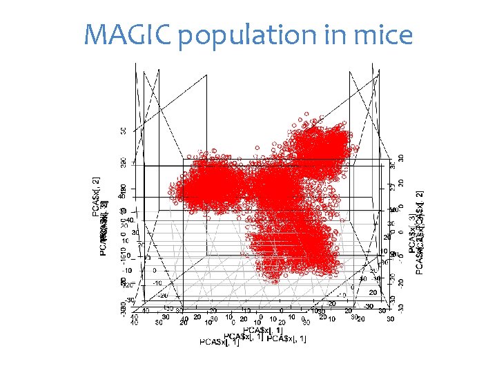
MAGIC population in mice

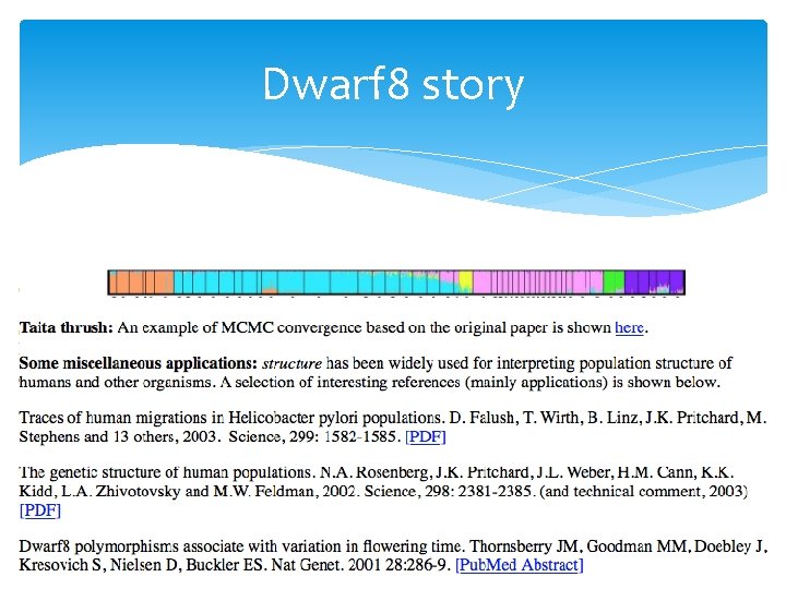
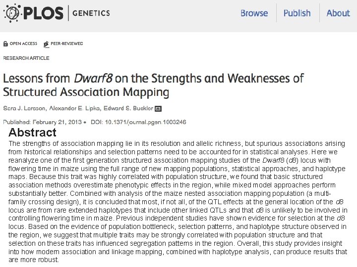
Dwarf 8 story

Abstract The strengths of association mapping lie in its resolution and allelic richness, but spurious associations arising from historical relationships and selection patterns need to be accounted for in statistical analyses. Here we reanalyze one of the first generation structured association mapping studies of the Dwarf 8 (d 8) locus with flowering time in maize using the full range of new mapping populations, statistical approaches, and haplotype maps. Because this trait was highly correlated with population structure, we found that basic structured association methods overestimate phenotypic effects in the region, while mixed model approaches perform substantially better. Combined with analysis of the maize nested association mapping population (a multifamily crossing design), it is concluded that most, if not all, of the QTL effects at the general location of the d 8 locus are from rare extended haplotypes that include other linked QTLs and that d 8 is unlikely to be involved in controlling flowering time in maize. Previous independent studies have shown evidence for selection at the d 8 locus. Based on the evidence of population bottleneck, selection patterns, and haplotype structure observed in the region, we suggest that multiple traits may be strongly correlated with population structure and that selection on these traits has influenced segregation patterns in the region. Overall, this study provides insight into how modern association and linkage mapping, combined with haplotype analysis, can produce results that are more robust.

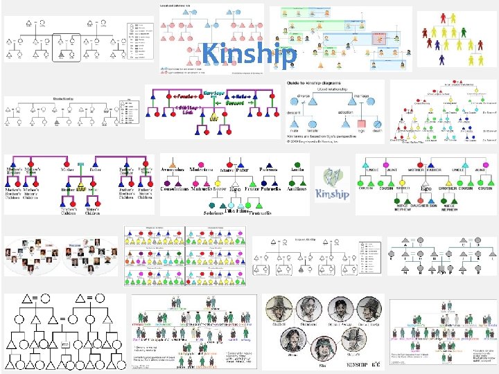
Kinship

Kinship Blood relationship Family ties, Blood ties, Common Ancestry Sharing of characteristics or origins.

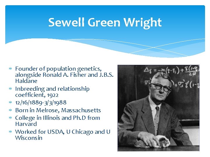
Sewell Green Wright Founder of population genetics, alongside Ronald A. Fisher and J. B. S. Haldane Inbreeding and relationship coefficient, 1922 12/16/1889 -3/3/1988 Born in Melrose, Massachusetts College in Illinois and Ph. D from Harvard Worked for USDA, U Chicago and U Wisconsin

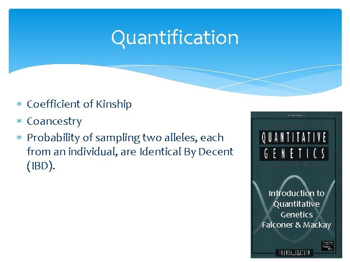
Quantification Coefficient of Kinship Coancestry Probability of sampling two alleles, each from an individual, are Identical By Decent (IBD). Introduction to Quantitative Genetics Falconer & Mackay

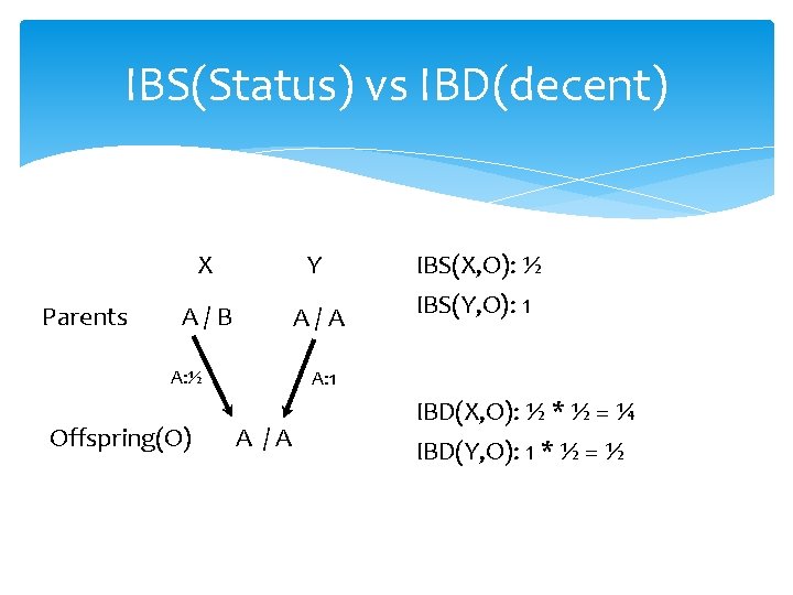
IBS(Status) vs IBD(decent) Parents X Y IBS(X, O): ½ A/B A/A IBS(Y, O): 1 A: ½ Offspring(O) A: 1 A /A IBD(X, O): ½ * ½ = ¼ IBD(Y, O): 1 * ½ = ½

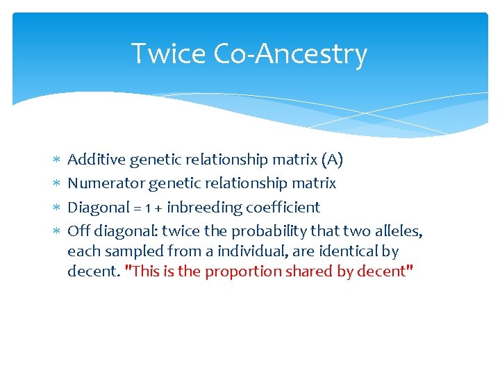
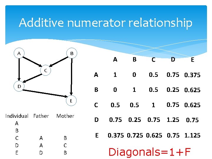
Twice Co-Ancestry Additive genetic relationship matrix (A) Numerator genetic relationship matrix Diagonal = 1 + inbreeding coefficient Off diagonal: twice the probability that two alleles, each sampled from a individual, are identical by decent. "This is the proportion shared by decent"

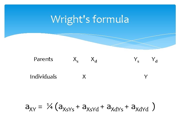
Wright's formula Parents Individuals Xs Xd X Ys Yd Y a. XY = ¼ (a. Xs. Ys + a. Xs. Yd + a. Xd. Ys + a. Xd. Yd )

Additive numerator relationship A B C D E Individual Father A B C A D A E D Mother B C B D A B C A 1 0 0. 5 0. 75 0. 375 B 0 1 0. 5 0. 25 0. 625 C 0. 5 1 0. 75 0. 625 D 0. 75 0. 25 0. 75 1. 25 0. 75 E 0. 375 0. 725 0. 625 0. 75 1. 125 Diagonals=1+F E

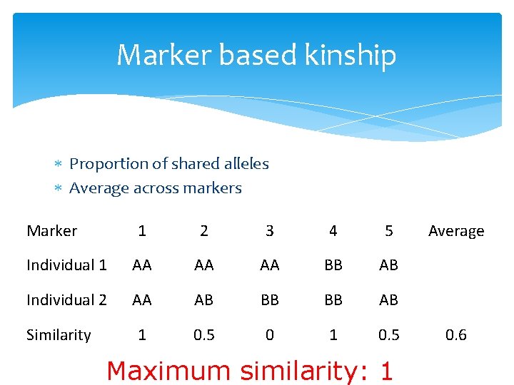
Marker based kinship Proportion of shared alleles Average across markers Marker 1 2 3 4 5 Individual 1 AA AA AA BB AB Individual 2 AA AB BB BB AB 1 0. 5 0 1 0. 5 Similarity Maximum similarity: 1 Average 0. 6

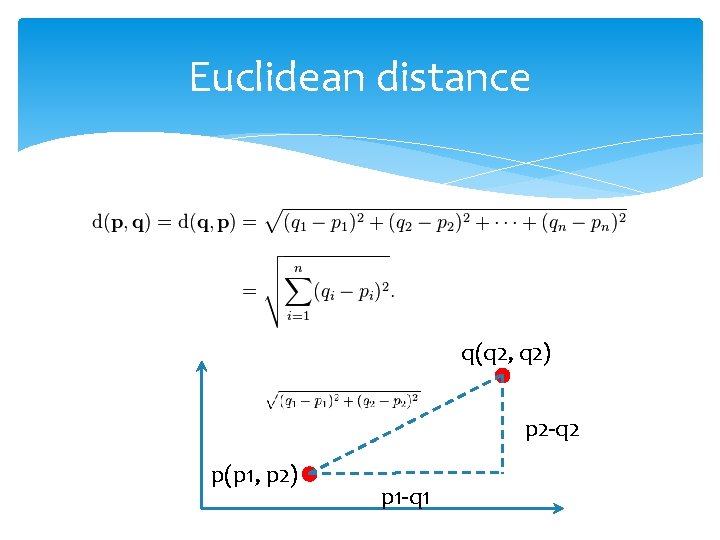
Euclidean distance q(q 2, q 2) p 2 -q 2 p(p 1, p 2) p 1 -q 1

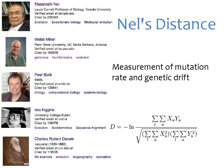
Nel's Distance Measurement of mutation rate and genetic drift

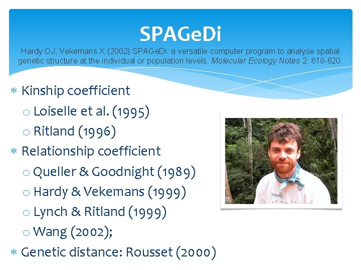
SPAGe. Di Hardy OJ, Vekemans X (2002) SPAGe. Di: a versatile computer program to analyse spatial genetic structure at the individual or population levels. Molecular Ecology Notes 2: 618 -620. Kinship coefficient o Loiselle et al. (1995) o Ritland (1996) Relationship coefficient o Queller & Goodnight (1989) o Hardy & Vekemans (1999) o Lynch & Ritland (1999) o Wang (2002); Genetic distance: Rousset (2000)

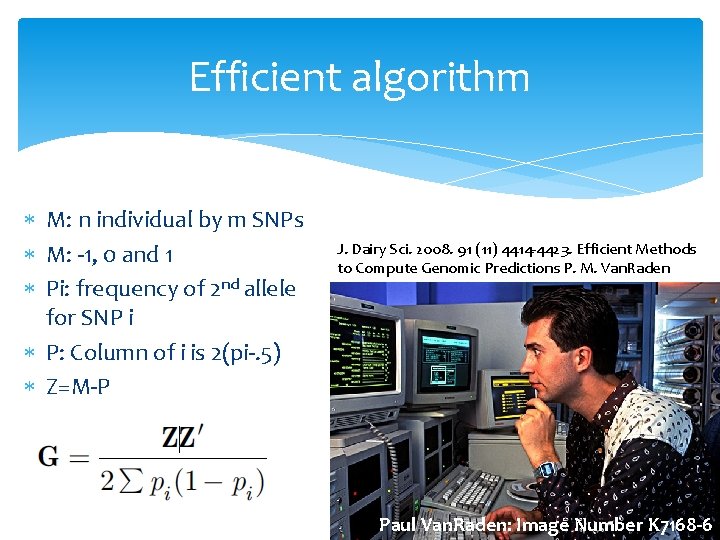
Efficient algorithm M: n individual by m SNPs M: -1, 0 and 1 Pi: frequency of 2 nd allele for SNP i P: Column of i is 2(pi-. 5) Z=M-P J. Dairy Sci. 2008. 91 (11) 4414 -4423. Efficient Methods to Compute Genomic Predictions P. M. Van. Raden Paul Van. Raden: Image Number K 7168 -6

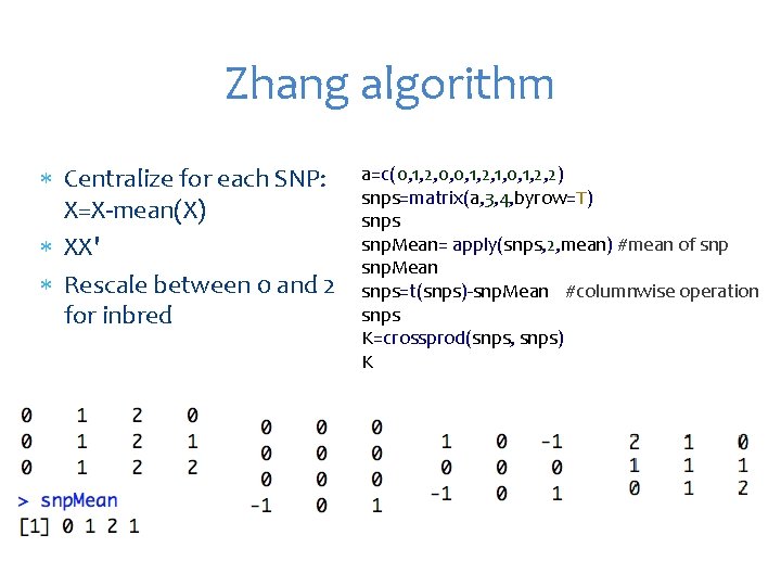
Zhang algorithm Centralize for each SNP: X=X-mean(X) XX' Rescale between 0 and 2 for inbred a=c(0, 1, 2, 0, 0, 1, 2, 1, 0, 1, 2, 2) snps=matrix(a, 3, 4, byrow=T) snps snp. Mean= apply(snps, 2, mean) #mean of snp. Mean snps=t(snps)-snp. Mean #columnwise operation snps K=crossprod(snps, snps) K

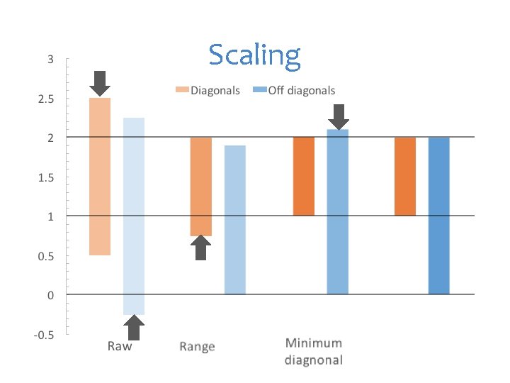
Scaling

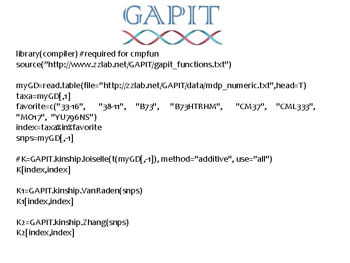
library(compiler) #required for cmpfun source("http: //www. zzlab. net/GAPIT/gapit_functions. txt") my. GD=read. table(file="http: //zzlab. net/GAPIT/data/mdp_numeric. txt", head=T) taxa=my. GD[, 1] favorite=c("33 -16", "38 -11", "B 73 HTRHM", "CM 37", "CML 333", "MO 17", "YU 796 NS") index=taxa%in%favorite snps=my. GD[, -1] #K=GAPIT. kinship. loiselle(t(my. GD[, -1]), method="additive", use="all") K[index, index] K 1=GAPIT. kinship. Van. Raden(snps) K 1[index, index] K 2=GAPIT. kinship. Zhang(snps) K 2[index, index]

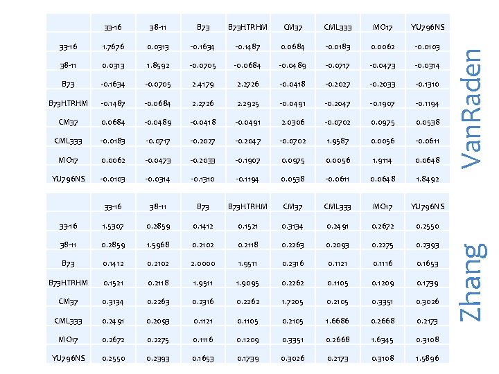
B 73 HTRHM CM 37 CML 333 MO 17 YU 796 NS 33 -16 1. 7676 0. 0313 -0. 1634 -0. 1487 0. 0684 -0. 0183 0. 0062 -0. 0103 38 -11 0. 0313 1. 8592 -0. 0705 -0. 0684 -0. 0489 -0. 0717 -0. 0473 -0. 0314 B 73 -0. 1634 -0. 0705 2. 4179 2. 2726 -0. 0418 -0. 2027 -0. 2033 -0. 1310 B 73 HTRHM -0. 1487 -0. 0684 2. 2726 2. 2925 -0. 0491 -0. 2047 -0. 1907 -0. 1194 CM 37 0. 0684 -0. 0489 -0. 0418 -0. 0491 2. 0306 -0. 0702 0. 0975 0. 0538 CML 333 -0. 0183 -0. 0717 -0. 2027 -0. 2047 -0. 0702 1. 9587 0. 0056 -0. 0611 MO 17 0. 0062 -0. 0473 -0. 2033 -0. 1907 0. 0975 0. 0056 1. 9114 0. 0648 YU 796 NS -0. 0103 -0. 0314 -0. 1310 -0. 1194 0. 0538 -0. 0611 0. 0648 1. 8492 33 -16 38 -11 B 73 HTRHM CM 37 CML 333 MO 17 YU 796 NS 33 -16 1. 5307 0. 2859 0. 1412 0. 1521 0. 3134 0. 2491 0. 2672 0. 2550 38 -11 0. 2859 1. 5968 0. 2102 0. 2118 0. 2263 0. 2093 0. 2275 0. 2393 B 73 0. 1412 0. 2102 2. 0000 1. 9511 0. 2316 0. 1121 0. 1116 0. 1653 B 73 HTRHM 0. 1521 0. 2118 1. 9511 1. 9095 0. 2262 0. 1105 0. 1209 0. 1739 CM 37 0. 3134 0. 2263 0. 2316 0. 2262 1. 7205 0. 2105 0. 3351 0. 3026 CML 333 0. 2491 0. 2093 0. 1121 0. 1105 0. 2105 1. 6686 0. 2668 0. 2173 MO 17 0. 2672 0. 2275 0. 1116 0. 1209 0. 3351 0. 2668 1. 6345 0. 3108 YU 796 NS 0. 2550 0. 2393 0. 1653 0. 1739 0. 3026 0. 2173 0. 3108 1. 5896 Van. Raden 38 -11 Zhang 33 -16

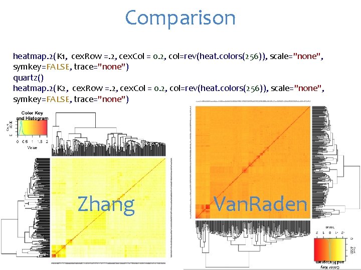
Comparison heatmap. 2(K 1, cex. Row =. 2, cex. Col = 0. 2, col=rev(heat. colors(256)), scale="none", symkey=FALSE, trace="none") quartz() heatmap. 2(K 2, cex. Row =. 2, cex. Col = 0. 2, col=rev(heat. colors(256)), scale="none", symkey=FALSE, trace="none") Zhang Van. Raden

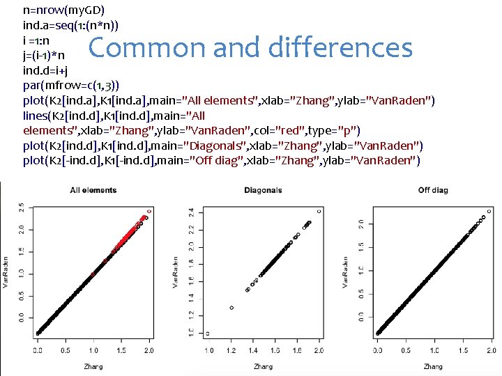
n=nrow(my. GD) ind. a=seq(1: (n*n)) i =1: n j=(i-1)*n ind. d=i+j par(mfrow=c(1, 3)) plot(K 2[ind. a], K 1[ind. a], main="All elements", xlab="Zhang", ylab="Van. Raden") lines(K 2[ind. d], K 1[ind. d], main="All elements", xlab="Zhang", ylab="Van. Raden", col="red", type="p") plot(K 2[ind. d], K 1[ind. d], main="Diagonals", xlab="Zhang", ylab="Van. Raden") plot(K 2[-ind. d], K 1[-ind. d], main="Off diag", xlab="Zhang", ylab="Van. Raden") Common and differences

Highlight Population structure is not enough Dwarf 8 story Kinship Additive Numerator Relationship Pedigree based Marker based