Imputation Sarah Medland Boulder 2019 What is imputation

Imputation Sarah Medland Boulder 2019

What is imputation? (Marchini & Howie 2010)

• 3 main reasons for imputation • Meta-analysis • Fine Mapping • Combining data from different chips • Other less common uses • sporadic missing data imputation • correction of genotyping errors • imputation of non-SNP variation

Combining data from different chips • Example • 750 individuals typed on the 370 K • 550 individuals typed on the 610 K • Power • MAF. 2 • SNP explaining 1% total variance • alpha 5 e-08 • N=1300, NCP 13. 07, power. 0331 • N=750, NCP 7. 54 , power. 0034 • N=550, NCP 5. 53 , power. 0009

Another way of looking at this

QQ-plot

Solution • Impute all individuals to a single reference based on the SNPs that overlap between the chips • Single distribution of NCP and power across all SNP • qq plot and manhattan describes the full sample with the same degree of accuracy

Imputation programs • minimac 3 • Impute 2 • Beagle – not frequently used • never use plink for imputation!

How do they compare • Similar accuracy • Similar features • Different data formats • minimac 3 –> custom vcf format • individual=row snp=column • Impute 2 –> snp=row individual=column • Different philosophies • Frequentist vs Bayesian

minimac 3 • http: //genome. sph. umich. edu/wiki/Minimac 3 • Built by Gonçalo Abecasis, Yun Li, Christian Fuchsberger and colleagues • Analysis options • SAIGE • Bolt. LMM • plink 2

Impute 2 • https: //mathgen. stats. ox. ac. uk/impute_v 2. html • http: //genome. sph. umich. edu/wiki/IMPUTE 2: _1000_Genomes_Imputation_Coo kbook • Built by Jonathan Marchini, Bryan Howie and colleges • Downstream analysis options • SNPtest • Quicktest

Timing & Memory from Das et al 2016 Prior to EAGLE 2

Options for imputation • DIY – Use a cookbook! http: //genome. sph. umich. edu/wiki/Minimac 3_Imputation_Cookbook OR http: //genome. sph. umich. edu/wiki/IMPUTE 2: _1000_Genomes_Imputation _Cookbook • UMich Imputation Server • https: //imputationserver. sph. umich. edu/ • Sanger Imputation Server • https: //imputation. sanger. ac. uk/

Today – discuss the 2 step approach Step 1 1000 Genomes Phase II haplotypes Step 2 Imputed GWAS genotypes

What is phasing • In this context it is really Haplotype Estimation • We take genotype data and try to reconstruct the haplotypes • Can use reference data to improve this estimation

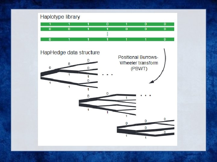
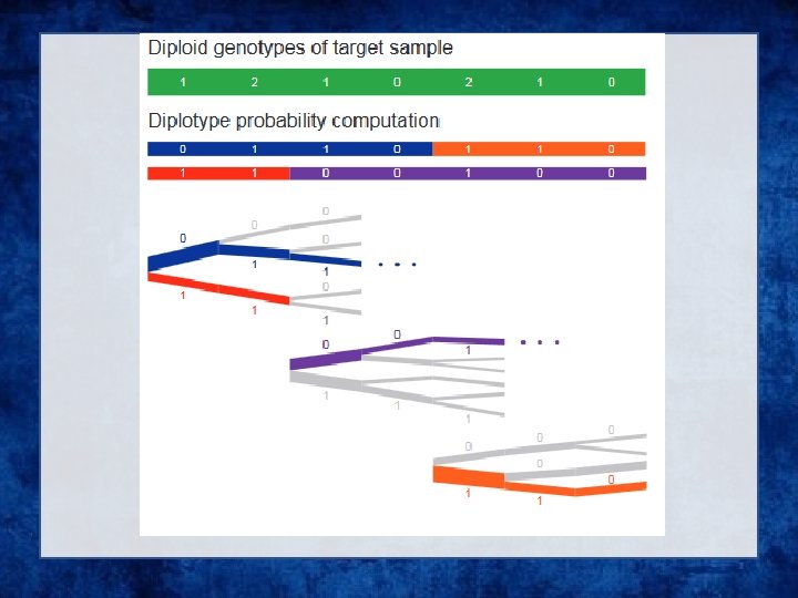
Phasing in Eagle • Input a target sample and a library of reference haplotypes • Selection of conditioning haplotypes. • Generation of Hap. Hedge data structure. • Exploration of the diplotype space.

Check your data i. Exclude snps with excessive missingness (>5%), low MAF (<1%), HWE violations (~P<10 -6), Mendelian errors ii. Drop strand ambiguous (palindromic) SNPs – ie A/T or C/G snps iii. Update build and alignment (b 37) iv. Output your data in the expected format for the phasing program you will use Check the naming convention for the program and reference you want to use rs 278405739 OR 22: 395704

Ambiguous SNPs (A/T and C/G)

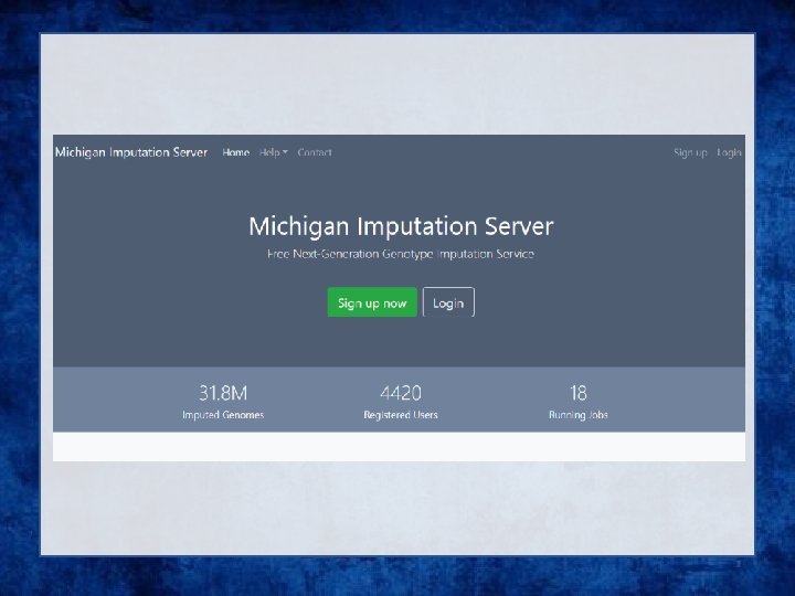
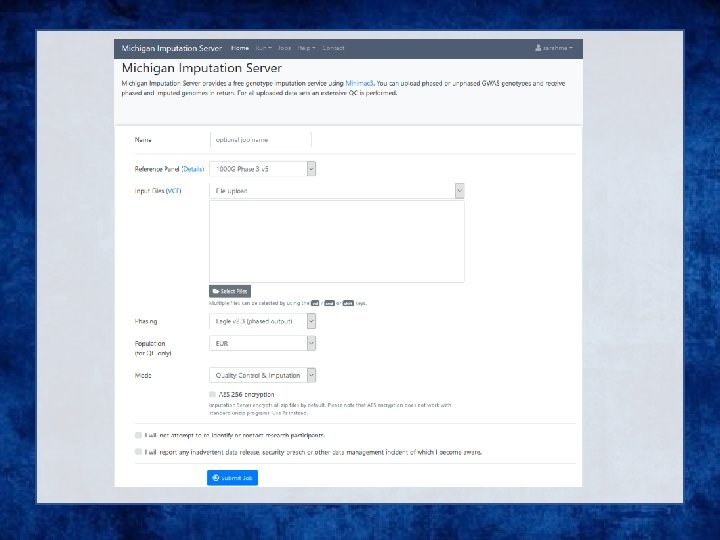
UMich imputation Server

Chose your reference • Current Publically Available References • Hap. Map. II (no phased X data officially released) • 1 KGP – phase 1 version v 3 • 1 KGP – phase 3 version v 5 • Future non-public references only available via custom imputation servers • HRC - 64, 976 haplotypes 39, 235, 157 SNPs • CAPPA – African American/Carabbean • Top. Med

References are in vcf format

Not all references are equal!! The Beagle and IMPUTE versions of the references contain variants that do not appear in the publically available 1 KGP data! The 1 KGP references still contain multiple locations with more than 1 variant & Multiple variants in more than one place!

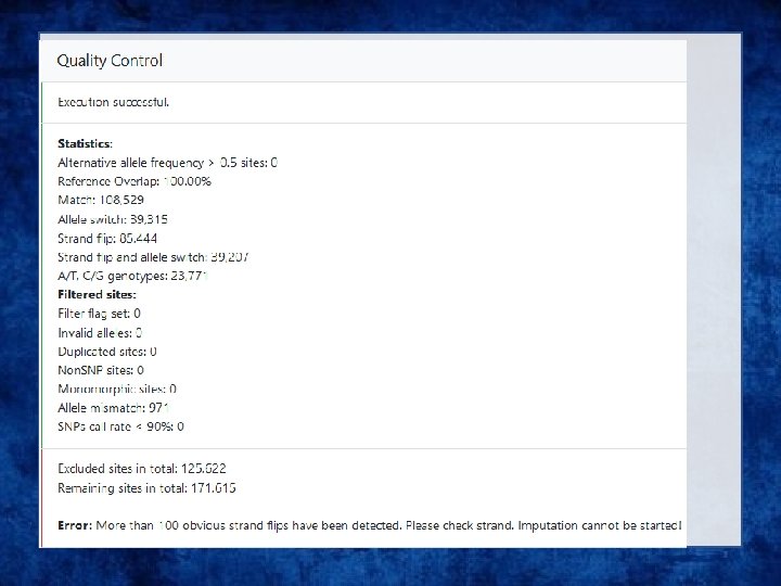
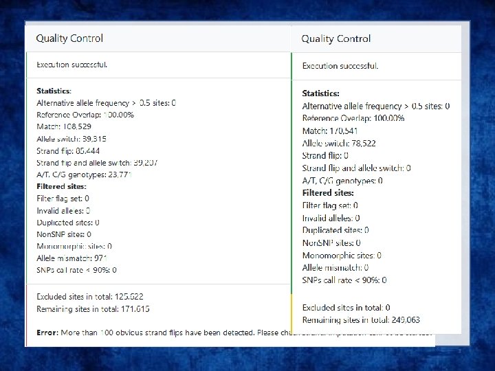
QC on the imputation server

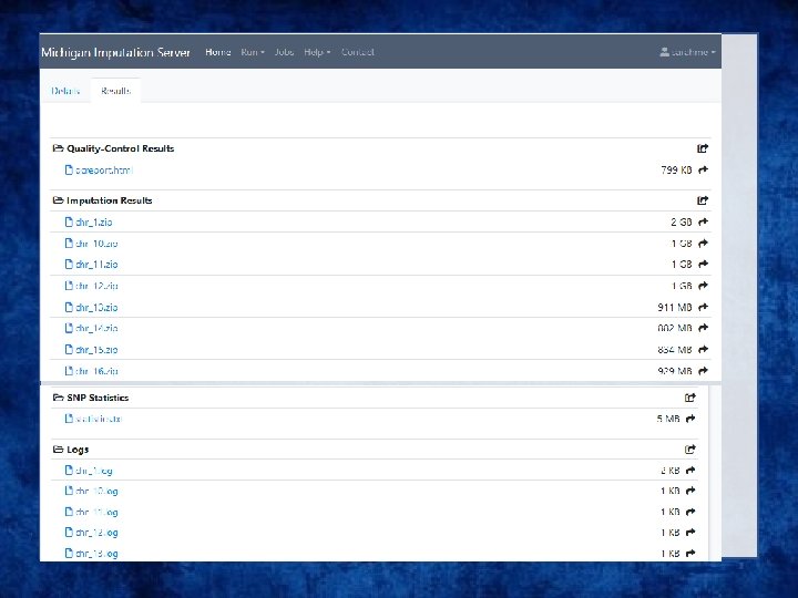
Output • Info files

Output • 3 main genotype output formats • Probs format (probability of AA AB and BB genotypes for each SNP) • Hard call or best guess (output as A C T or G allele codes) • Dosage data (most common – 1 number per SNP, 1 -2)

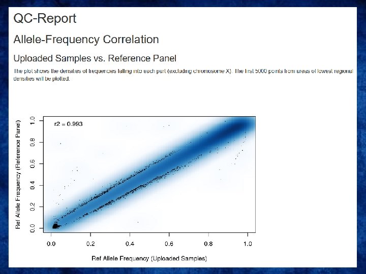
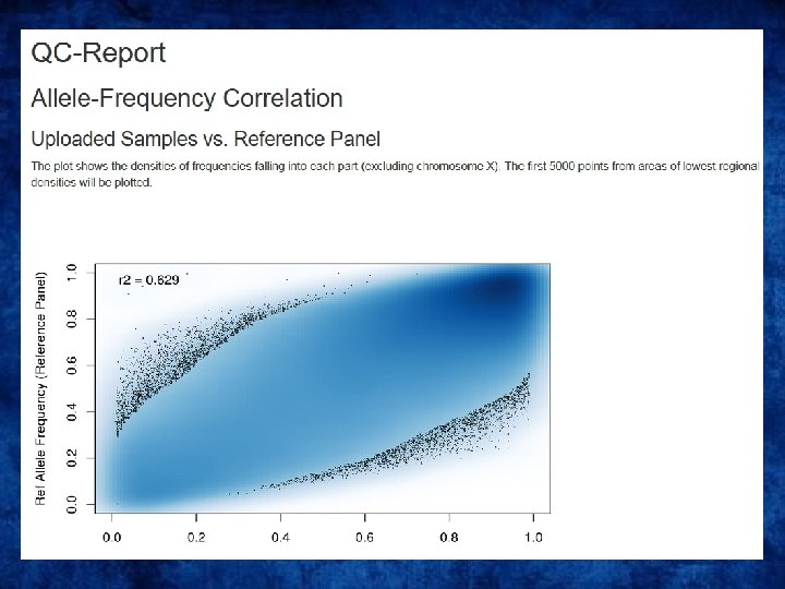
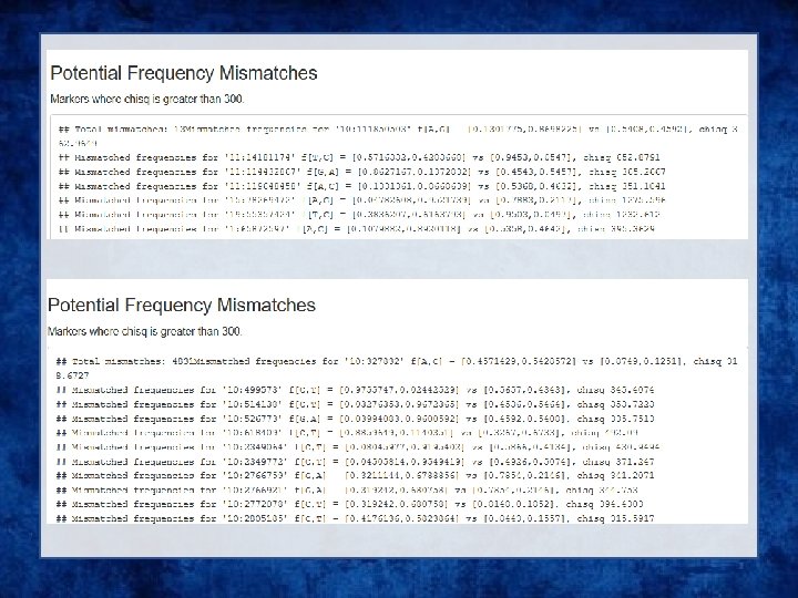
Post imputation QC • After imputation you need to check that it worked and the data look ok • Things to check • Plot r 2 across each chromosome look to see where it drops off • Plot MAF-reference MAF

Issue – the r 2 metrics differ between imputation programs

• In general fairly close correlation • rsq/ Proper. Info/ allelic Rsq • 1 = no uncertainty • 0 = complete uncertainty • . 8 on 1000 individuals = amount of data at the SNP is equivalent to a set of perfectly observed genotype data in a sample size of 800 individuals • Note Mach uses an empirical Rsq (observed var/exp var) and can go above 1

Good imputation Bad imputation

Post imputation QC • Next run GWAS for a trait – ideally continuous, calculate lambda and plot: • QQ • Manhattan • SE vs N • P vs Z • Run the same trait on the observed genotypes – plot imputed vs observed

If you are running analyses for a consortium they will probably ask you to analyse all variants regardless of whether they pass QC or not… (If you are setting up a meta-analysis consider allowing cohorts to ignore variants with MAF <. 5% and low r 2 – it will save you a lot of time)

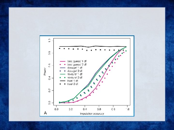
Choices of analysis methods

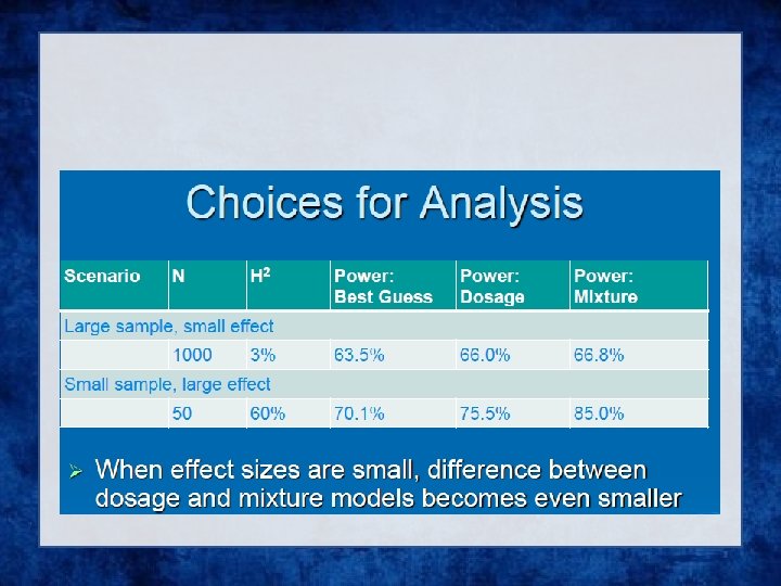
Analysis of Imputed data using SAIGE

Why SAIGE PROS • Fast • Low memory • Can cope with UKB size data • Correctly models zygosity and relatedness • Continuous or Binary CONS • 2 stages • 1 trait at a time • Phenotypes and covariates all in one file

Step 1 • Runs the LMM and creates a pre-processed r data file Rscript step 1_fit. NULLGLMM. R --plink. File=sparse --pheno. File=pheno. AD. txt --pheno. Col=AD --covar. Col. List=PC 1, PC 2, PC 3, PC 4 --sample. IDColinpheno. File=FID_IID --trait. Type=binary --output. Prefix=AD > AD. log

Phenotype/Covariate file • Simple format – headers, space delim • Binary traits are 0/1 • Need to join FID and IID with an underscore _ as this is the ID format in the imputed data

Plink (hard call) genotypes for relatedness estimation • Doesn’t need to be all available data – can be a sparse file • Todays files contains ~75, 000 snps plink --bfile QCed --indep-pairwise 10000 kb 5. 2 --out prune plink --bfile QCed --extract prune. in --make-bed --out sparse

Step 1 • Runs the LMM and creates a pre-processed r data file Rscript step 1_fit. NULLGLMM. R --plink. File=sparse --pheno. File=pheno. AD. txt --pheno. Col=AD --covar. Col. List=PC 1, PC 2, PC 3, PC 4 --sample. IDColinpheno. File=FID_IID --trait. Type=binary --output. Prefix=AD > AD. log

It will make 4 files • Log, Rda, variance. Ratio. txt, _30 markers. SAIGE. results. txt • • R load("example. rda") names(modglmm) modglmm$theta • #theta: a vector of length 2. The first element is the dispersion parameter estimate and the second one is the variance component parameter estimate • #coefficients: fixed effect parameter estimates • #linear. predictors: a vector of length N (N is the sample size) containing linear predictors • #fitted. values: a vector of length N (N is the sample size) containing fitted mean values on the original scale • #Y: a vector of length N (N is the sample size) containing final working vector • #residuals: a vector of length N (N is the sample size) containing residuals on the original scale

Step 2 Rscript step 2_SPAtests. R --vcf. File=chr 19. dose. vcf. gz --vcf. File. Index=chr 19. dose. vcf. gz. tbi --sample. File=sample. txt --vcf. Field=DS --chrom=19 --min. MAF=0. 01 --min. MAC=5 --GMMATmodel. File=AD. rda --variance. Ratio. File=AD. variance. Ratio. txt --SAIGEOutput. File=AD. chr 19. SAIGE. txt --num. Lines. Output=2 --Is. Output. AFin. Case. Ctrl=TRUE &> AD. chr 19. SAIGE. log

Output CHR: chromosome POS: genome position SNPID: variant ID Allele 1: Ref allele Allele 2: Alt allele AC_Allele 2: allele count of Alt allele AF_Allele 2: allele freq of Alt allele N: sample size BETA: effect size of A 2 SE: standard error of BETA Tstat: score statistic p. value: p value with SPA applied p. value. NA: p value when SPA is not applied Is. SPA. converge: whether SPA is converged or not var. T: estimated variance of score statistic with sample related incorporated var. Tstar: variance of score statistic without sample related incorporated

Merge the GWAS results with the R 2 from the imputation files and keep only those results with r 2 >= 0. 6 (i. e. good imputation quality) #### Merge results GWAS with imputed information file and filter by R 2 >= 6 (the results have been filtered by MAF before) # Extract columns of interest in GWAS results: CHR POS SNPID Allele 1 Allele 2 AF_Allele 2 N BETA SE Tstat p. value zcat AD. chr 19. SAIGE. txt. gz | awk '{print $1, $2, $3, $4, $5, $7, $8, $9, $10, $11, $12}' > temp_AD. chr 19. results. txt # Extract columns of interest in imputation information: SNP Rsq zcat. . /saige/chr 19. info. gz | awk '{print $1, $7}' > temp_chr 19. info. txt # Merge information from the GWAS and R 2 awk 'NR==FNR{a[$1]=$2; next} $3 in a{print $0, a[$3]}' temp_chr 19. info. txt temp_AD. chr 19. results. txt > temp # Filer by R 2 >= 0. 6 and put the header echo 'CHR POS SNPID Allele 1 Allele 2 AF_Allele 2 N BETA SE Tstat p. value Rsq' > AD. chr 19. results. QC. txt awk '{if ($12>=0. 6) print $0}' temp >> AD. chr 19. results. QC. txt #### Plot the results: Manhattan plot and regional plot awk '{if (NR>1) print $1, $2, $11}' temp_AD. chr 19. results. QC. txt > temp_plot. AD. chr 19. txt sort -k 11 -g temp_AD. chr 19. results. QC. txt | head # lowest p-value at 19: 45422946 , p = 9. 3515193823689 e-16 awk '{if (NR==1) print $1, $2, $3, $11; else if ($2>= 44922946 && $2<= 45922946) print $1, $2, "chr"$3, $11}' AD. chr 19. results. QC. txt > temp_ld. AD. chr 19. txt

Imputed results (Manhattan plot only chr 19)

Remember the genotyped results!

And Compare… Genotyped Imputed

Imputed results (regional plot)

And Compare… Genotyped Imputed

Questions?

Extra slides

Step 1 – How to phase Data is usually broken into manageable chunks ~20 Mb Each phased independently. /eagle --vcf. Ref HRC. r 11. GRCh 37. chr 20. shapeit 3. mac 5. aa. genotypes. bcf --vcf. Target chunk_20_000001_0020000000. vcf. gz --genetic. Map. File genetic_map_chr 20_combined_b 37. txt --out. Prefix chunk_20_000001_0020000000. phased --bp. Start 1 --bp. End 25000000 --chrom 20 --allow. Ref. Alt. Swap

Step 2 - Imputation • Compares the phased data to the references and infers the missing genotypes. Calculate accuracy metrics. /Minimac 3 --ref. Haps HRC. r 11. GRCh 37. chr 1. shapeit 3. mac 5. aa. genotypes. m 3 vcf. gz --haps chunk_1_000001_0020000000. phased. vcf --start 1 --end 20000000 --window 500000 --prefix chunk_1_000001_0020000000 --chr 20 --no. Phone. Home --format GT, DS, GP --all. Typed. Sites

Phasing in Eagle • Input a target sample and a library of reference haplotypes • Selection of conditioning haplotypes. Eagle 2 first identifies a subset of 10, 000 conditioning haplotypes by ranking reference haplotypes according to the number of discrepancies between each reference haplotype and the homozygous genotypes of the target sample.

• Generation of Hap. Hedge data structure. Eagle 2 next generates a Hap. Hedge data structure on the selected conditioning haplotypes. The Hap. Hedge encodes a sequence of haplo- type prefix trees (i. e. , binary trees on haplotype prefixes) rooted at a sequence of starting positions along the chromosome, thus enabling fast lookup of haplotype frequencies

• Exploration of the diplotype space. Having prepared a Hap. Hedge of conditioning haplotypes, Eagle 2 performs phasing using a hidden Markov model Consolidates reference haplotypes sharing common prefixes reducing computation.