Stata in Space An example for the econometric

Stata in Space: An example for the econometric analysis of spatially explicit raster data --- Daniel Müller --Institute of Agricultural Economics and Social Sciences Humboldt University Berlin -- August, 12 th, 2003

Outline 1. Introduction 2. Spatial data analysis 3. Data preparation 4. The empirical example 5. Econometric estimation 6. Export of results and geovisualization

Introduction 1. Socioeconomic data usually exist for (discrete) social entities, rarely explicitly linked to location (georeferenced) 2. ‘Natural’ data: often continuous (rainfall, slope, elevation) and georeferenced 3. Integration of both data sources can provide additional insights 1. Allows to understand spatial patterns & processes 2. Knowing the where can help us infer the why

Spatial data analysis 1. Spatial analysis is the analysis of data linked to location (spatial data) 2. Why analysis of spatial data ? 1. Variables of interest vary in space 2. Location matters! 3. Spatial analysis can provide important insights: 1. geographical targeting of investments 2. diffusion of technologies 3. causes and consequences of land-use change

Spatial data analysis What’s special about spatial data ? => Location matters !!! => Tobler’s 1 st law of geography (1979): “Everything is related to everything else, but near things are more related than distant things. ” => Spatial effects: - spatial autocorrelation - spatial heterogeneity 17 -Jul-2002 danielix@gmx. net

Spatial data analysis Peculiarities in space: Spatial effects 1. Spatial autocorrelation - Coincidence of value similarity with locational similarity - Second dimension adds mathematical complexity (multiple directions) 2. Spatial heterogeneity - Each location is unique - Units of observations not homogeneous across space - Structural instability over space, e. g. heteroskedasticity

Spatial data analysis Peculiarities in space: spatial effects [2] Spatial effects due to: - interactions among neighboring agents data from different sources different sample designs varying aggregation rules “Spatial relationships among observations can result in unreliable estimates and misguided statistical inference of the parameters. ” (Anselin 1988). => Corrections necessary

Spatial data analysis Geographic Information Systems (GIS): - Compile, store, manipulate, analyse, visualize spatial data - Consist of hardware, software, data and procedures - Data models: vector & raster

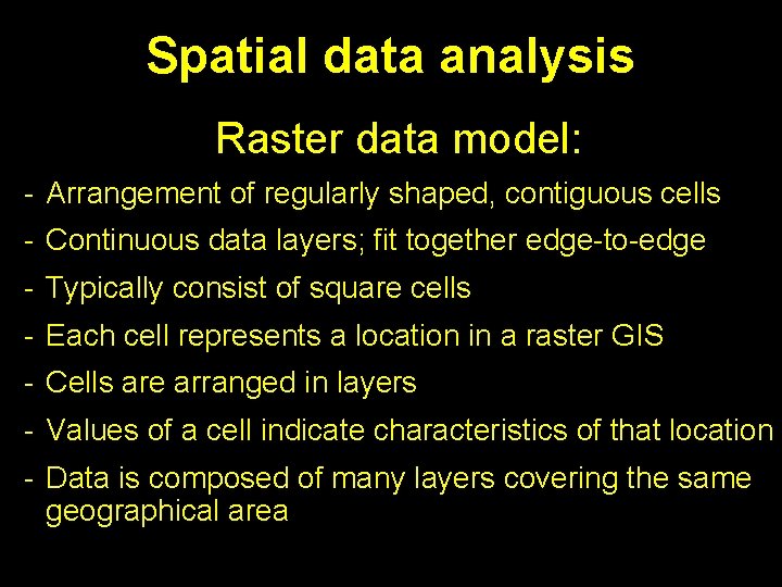
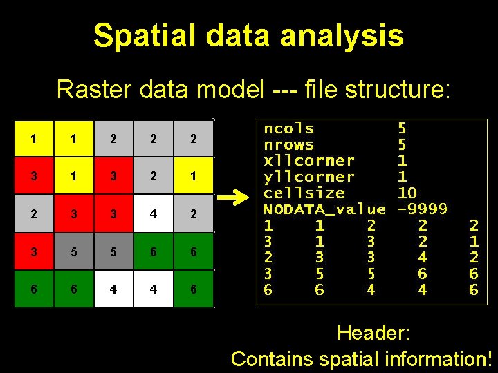
Spatial data analysis Raster data model: - Arrangement of regularly shaped, contiguous cells - Continuous data layers; fit together edge-to-edge - Typically consist of square cells - Each cell represents a location in a raster GIS - Cells are arranged in layers - Values of a cell indicate characteristics of that location - Data is composed of many layers covering the same geographical area

Spatial data analysis Raster data model --- file structure: 1 1 2 2 2 3 1 3 2 1 2 3 3 4 2 3 5 5 6 6 4 4 6 Header: Contains spatial information!

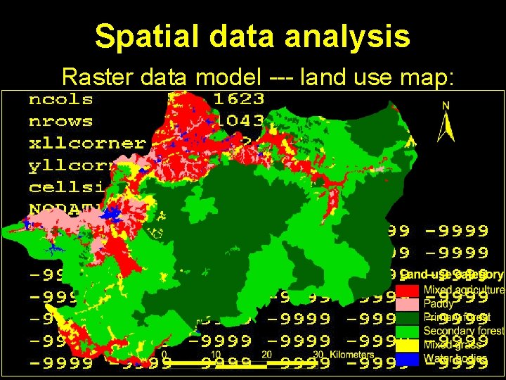
Spatial data analysis Raster data model --- land use map:

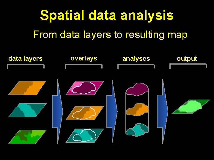
Spatial data analysis From data layers to resulting map data layers overlays analyses output

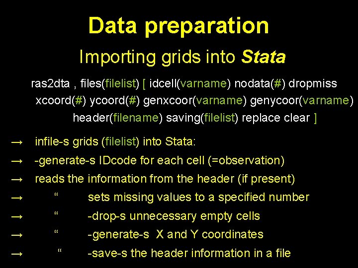
Data preparation Importing grids into Stata ras 2 dta , files(filelist) [ idcell(varname) nodata(#) dropmiss xcoord(#) ycoord(#) genxcoor(varname) genycoor(varname) header(filename) saving(filelist) replace clear ] → infile-s grids (filelist) into Stata: → -generate-s IDcode for each cell (=observation) → reads the information from the header (if present) → “ sets missing values to a specified number → “ -drop-s unnecessary empty cells → “ -generate-s X and Y coordinates → “ -save-s the header information in a file

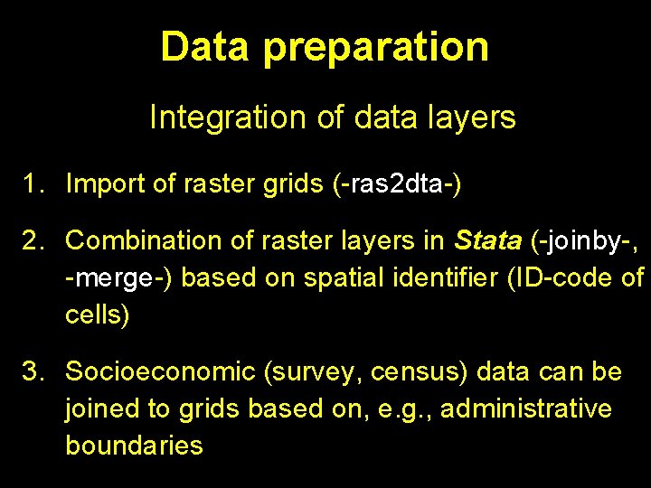
Data preparation Integration of data layers 1. Import of raster grids (-ras 2 dta-) 2. Combination of raster layers in Stata (-joinby-, -merge-) based on spatial identifier (ID-code of cells) 3. Socioeconomic (survey, census) data can be joined to grids based on, e. g. , administrative boundaries

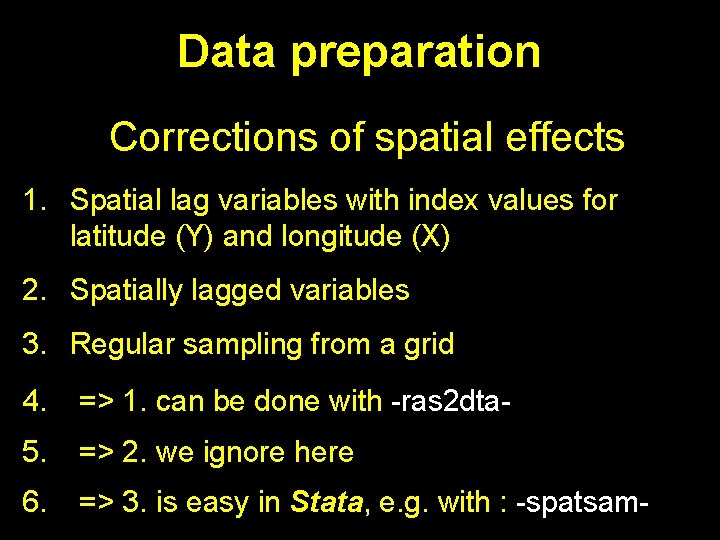
Data preparation Corrections of spatial effects 1. Spatial lag variables with index values for latitude (Y) and longitude (X) 2. Spatially lagged variables 3. Regular sampling from a grid 4. => 1. can be done with -ras 2 dta- 5. => 2. we ignore here 6. => 3. is easy in Stata, e. g. with : -spatsam-

Data preparation spatsam , gap(#) xcoord(varname) ycoord(varname) [ saving(filename) norestore noseed replace ] Basically that‘s: keep if (xcoord / gap) == int (xcoord / gap) & (ycoord / gap) == int (ycoord / gap) Therefore, only every #-th observation in X and Y direction is kept in the sample.

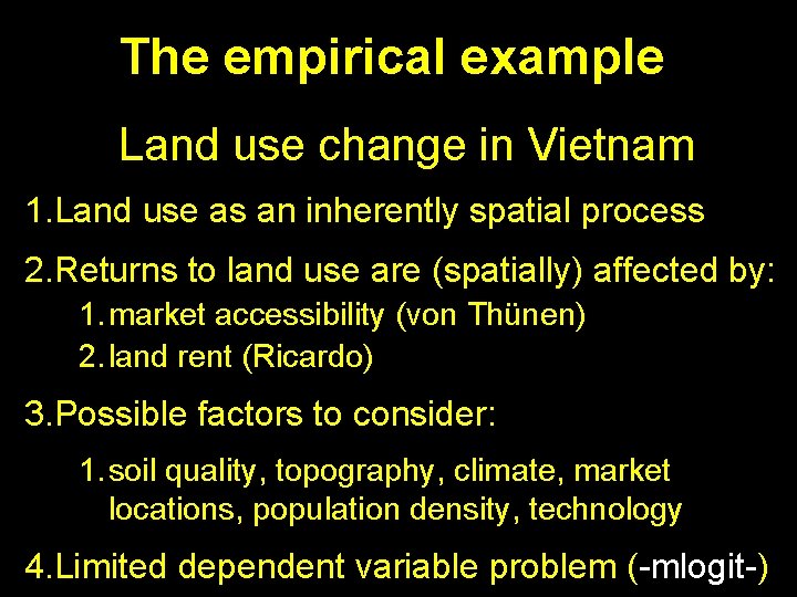
The empirical example Land use change in Vietnam 1. Land use as an inherently spatial process 2. Returns to land use are (spatially) affected by: 1. market accessibility (von Thünen) 2. land rent (Ricardo) 3. Possible factors to consider: 1. soil quality, topography, climate, market locations, population density, technology 4. Limited dependent variable problem (-mlogit-)

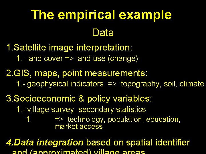
The empirical example Data 1. Satellite image interpretation: 1. - land cover => land use (change) 2. GIS, maps, point measurements: 1. - geophysical indicators => topography, soil, climate 3. Socioeconomic & policy variables: 1. - village survey, secondary statistics 1. => technology, population, education, market access 4. Data integration based on spatial identifier

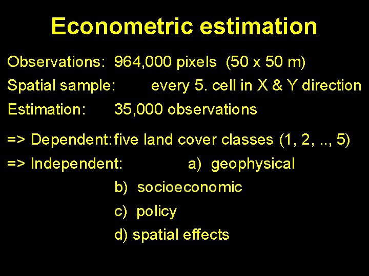
Econometric estimation Observations: 964, 000 pixels (50 x 50 m) Spatial sample: every 5. cell in X & Y direction Estimation: 35, 000 observations => Dependent: five land cover classes (1, 2, . . , 5) => Independent: a) geophysical b) socioeconomic c) policy d) spatial effects

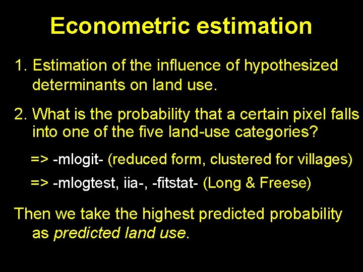
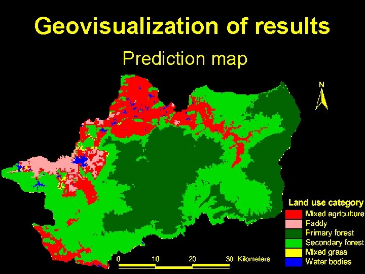
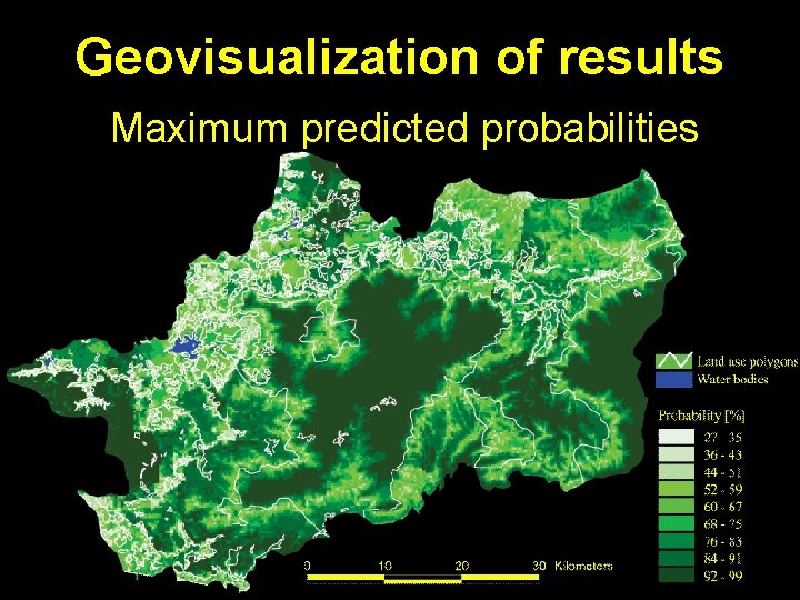
Econometric estimation 1. Estimation of the influence of hypothesized determinants on land use. 2. What is the probability that a certain pixel falls into one of the five land-use categories? => -mlogit- (reduced form, clustered for villages) => -mlogtest, iia-, -fitstat- (Long & Freese) Then we take the highest predicted probability as predicted land use.

Export of results Outputting results from Stata dta 2 ras [varlist], xcoord(#) ycoord(#) cellsize(#) [ header(filename) idcell(varname) nodata(#) xllcorner(#) yllcorner(#) saving(varlist) replace ] → writes header in front of file with the information from xcoord(#) ycoord(#) cellsize(#) or header(); (optionally) nodata(#) xllcorner(#) yllcorner(#) → then the results can be mapped in the GIS

Geovisualization of results Prediction map

Geovisualization of results Maximum predicted probabilities

Thank you ! Questions, comments and critique welcome ! ______________ © Daniel Müller (danielix@gmx. net) Institute of Agricultural Economics and Social Sciences ---- Humboldt University Berlin ---Stata ados available for download at: http: //amor. cms. hu-berlin. de/~muelleda