Product Variety and Quality under Monopoly 1 Introduction

Product Variety and Quality under Monopoly 1

Introduction • Most firms sell more than one product • Products are differentiated in different ways – horizontally • goods of similar quality targeted at consumers of different types – how is variety determined? – is there too much variety – vertically • consumers agree on quality • differ on willingness to pay for quality – how is quality of goods being offered determined? 2

Horizontal product differentiation • Suppose that consumers differ in their tastes – firm has to decide how best to serve different types of consumer – offer products with different characteristics but similar qualities • This is horizontal product differentiation – firm designs products that appeal to different types of consumer – products are of (roughly) similar quality • Questions: – how many products? – of what type? – how do we model this problem? 3

A spatial approach to product variety • The spatial model (Hotelling) is useful to consider – pricing – design – variety • Has a much richer application as a model of product differentiation – “location” can be thought of in • space (geography) • time (departure times of planes, buses, trains) • product characteristics (design and variety) – consumers prefer products that are “close” to their preferred types in space, or time or characteristics 4

A Spatial approach to product variety 2 • Assume N consumers living equally spaced along Main Street – 1 mile long. • Monopolist must decide how best to supply these consumers • Consumers buy exactly one unit provided that price plus transport costs is less than V. • Consumers incur there-and-back transport costs of t per mile • The monopolist operates one shop – reasonable to expect that this is located at the center of Main Street 5

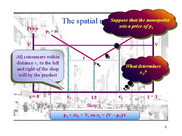
Suppose that the monopolist The spatial model Price sets a price of. Price p 1 + tx p 1 + t. x V V All consumers within distance x 1 to the left and right of the shop will by the product z=0 t x 1 t p 1 1/2 What determines x 1? x 1 z=1 Shop 1 + tx 1 = V, so x 1 = (V – p 1)/t 6

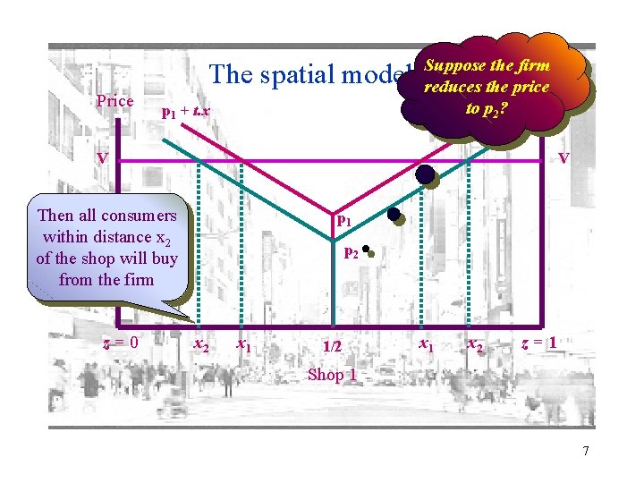
Suppose the firm reduces the price Price p 1 +tot. xp 2? The spatial model 2 Price p 1 + t. x V V Then all consumers within distance x 2 of the shop will buy from the firm z=0 p 1 p 2 x 1 1/2 x 1 x 2 z=1 Shop 1 7

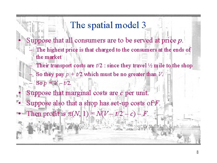
The spatial model 3 • Suppose that all consumers are to be served at price p. – The highest price is that charged to the consumers at the ends of the market – Their transport costs are t/2 : since they travel ½ mile to the shop – So they pay p + t/2 which must be no greater than V. – So p = V – t/2. • Suppose that marginal costs are c per unit. • Suppose also that a shop has set-up costs of F. • Then profit is p(N, 1) = N(V – t/2 – c) – F. 8

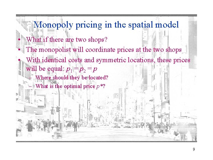
Monopoly pricing in the spatial model • What if there are two shops? • The monopolist will coordinate prices at the two shops • With identical costs and symmetric locations, these prices will be equal: p 1 = p 2 = p – Where should they be located? – What is the optimal price p*? 9

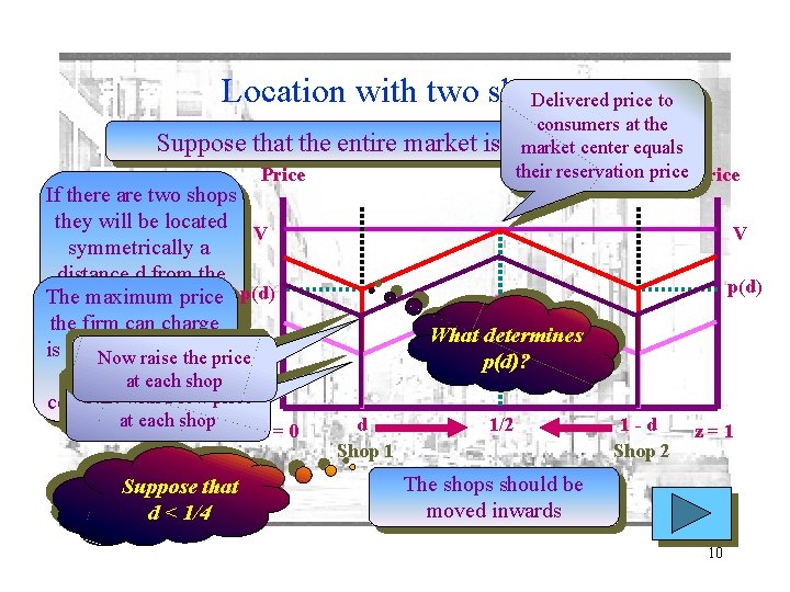
Location with two shops Delivered price to Suppose that the entire market is Price If there are two shops they will be located V symmetrically a distance d from the The maximumofprice end-points the p(d) the firmmarket can charge is determined Now raisebythethe price consumers at the at each shop Start with a low center of the marketprice at each shop Suppose that d < 1/4 z=0 consumers at the tomarket be served center equals their reservation price Price V p(d) What determines p(d)? d Shop 1 1/2 1 -d Shop 2 z=1 The shops should be moved inwards 10

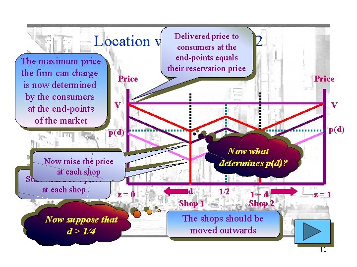
Delivered price to consumers at the end-points equals their reservation price Location with two shops 2 The maximum price the firm can charge is now determined by the consumers at the end-points of the market Price V V p(d) Now raise the price at each shop Start with a low price at each shop Now suppose that d > 1/4 Now what determines p(d)? z=0 d Shop 1 1/2 1 -d Shop 2 z=1 The shops should be moved outwards 11

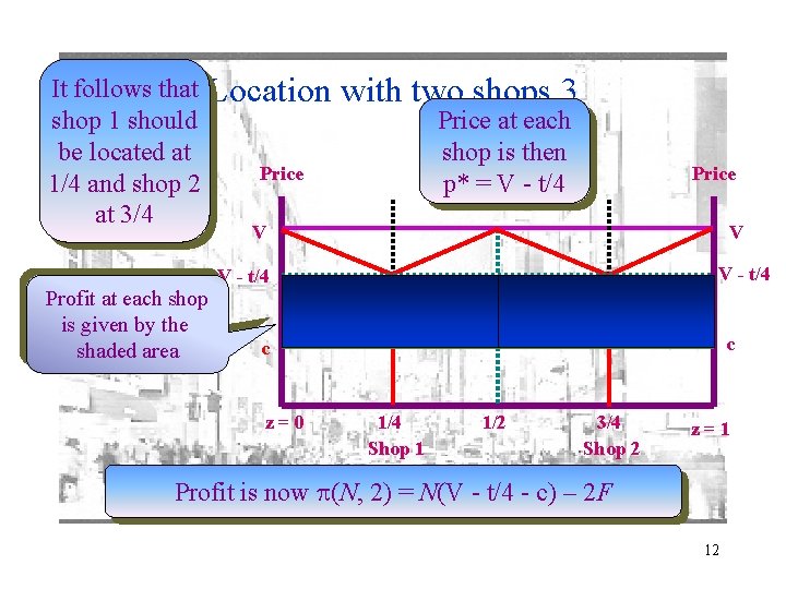
It follows that Location shop 1 should be located at Price 1/4 and shop 2 at 3/4 with two shops 3 Price at each shop is then p* = V - t/4 Price V V V - t/4 Profit at each shop is given by the shaded area c c z=0 1/4 Shop 1 1/2 3/4 Shop 2 z=1 Profit is now p(N, 2) = N(V - t/4 - c) – 2 F 12

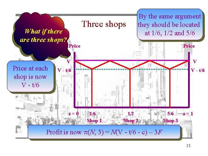
What if there are three shops? Price at each shop is now V - t/6 Three shops By the same argument they should be located at 1/6, 1/2 and 5/6 Price V V V - t/6 z=0 V - t/6 1/6 Shop 1 1/2 Shop 2 5/6 z=1 Shop 3 Profit is now p(N, 3) = N(V - t/6 - c) – 3 F 13

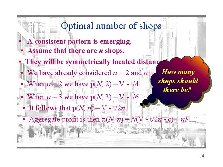
Optimal number of shops • A consistent pattern is emerging. • Assume that there are n shops. • They will be symmetrically located distance 1/n apart. • We have already considered n = 2 and n = 3. How many shops should • When n = 2 we have p(N, 2) = V - t/4 there be? • When n = 3 we have p(N, 3) = V - t/6 • It follows that p(N, n) = V - t/2 n • Aggregate profit is then p(N, n) = N(V - t/2 n - c) – n. F 14

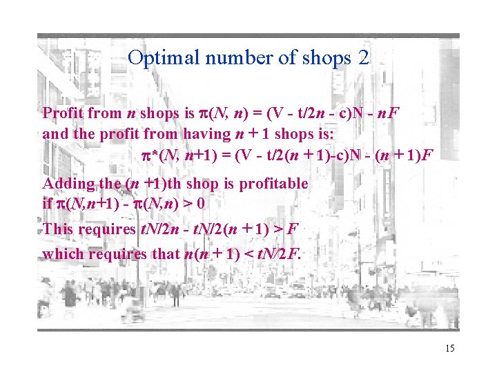
Optimal number of shops 2 Profit from n shops is p(N, n) = (V - t/2 n - c)N - n. F and the profit from having n + 1 shops is: p*(N, n+1) = (V - t/2(n + 1)-c)N - (n + 1)F Adding the (n +1)th shop is profitable if p(N, n+1) - p(N, n) > 0 This requires t. N/2 n - t. N/2(n + 1) > F which requires that n(n + 1) < t. N/2 F. 15

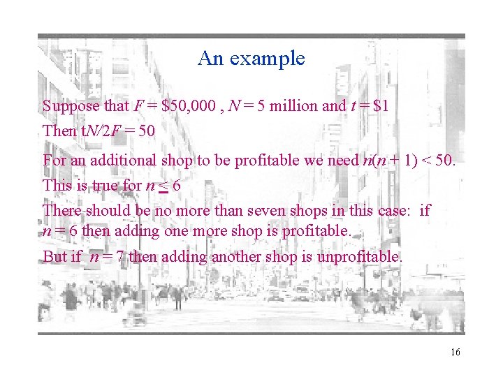
An example Suppose that F = $50, 000 , N = 5 million and t = $1 Then t. N/2 F = 50 For an additional shop to be profitable we need n(n + 1) < 50. This is true for n < 6 There should be no more than seven shops in this case: if n = 6 then adding one more shop is profitable. But if n = 7 then adding another shop is unprofitable. 16

Some intuition • What does the condition on n tell us? • Simply, we should expect to find greater product variety when: – there are many consumers. – set-up costs of increasing product variety are low. – consumers have strong preferences over product characteristics and differ in these • consumers are unwilling to buy a product if it is not “very close” to their most preferred product 17

How much of the market to supply • Should the whole market be served? – Suppose not. Then each shop has a local monopoly – Each shop sells to consumers within distance r – How is r determined? • • it must be that p + tr = V so r = (V – p)/t so total demand is 2 N(V – p)/t profit to each shop is then p = 2 N(p – c)(V – p)/t – F differentiate with respect to p and set to zero: dp/dp = 2 N(V – 2 p + c)/t = 0 So the optimal price at each shop is p* = (V + c)/2 If all consumers are served price is p(N, n) = V – t/2 n – Only part of the market should be served if p(N, n)< p* – This implies that V < c + t/n. 18

Partial market supply • If c + t/n > V supply only part of the market and set price p* = (V + c)/2 • If c + t/n < V supply the whole market and set price p(N, n) = V – t/2 n • Supply only part of the market: – if the consumer reservation price is low relative to marginal production costs and transport costs – if there are very few outlets 19

Are there too Social optimum many shops or What number of shops maximizes total surplus? too few? Total surplus is consumer surplus profit Consumer surplus is total willingness to pay minus total revenue Profit is total revenue minus total cost Total surplus is then total willingness to pay minus total costs Total willingness to pay by consumers is N. V Total surplus is therefore NV - Total Cost So what is Total Cost? 20

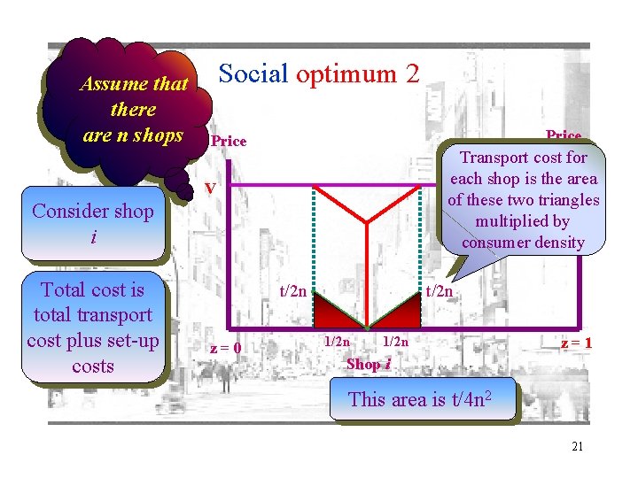
Assume that there are n shops Social optimum 2 Price Transport cost for each shop is the area V of these two triangles multiplied by consumer density V Consider shop i Total cost is total transport cost plus set-up costs t/2 n z=0 t/2 n 1/2 n z=1 Shop i This area is t/4 n 2 21

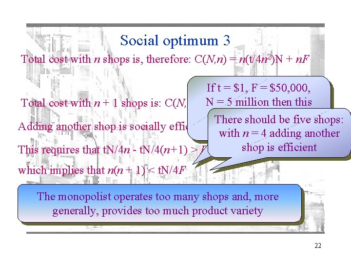
Social optimum 3 Total cost with n shops is, therefore: C(N, n) = n(t/4 n 2)N + n. F If = t =t. N/4 n $1, F+=n. F $50, 000, 5 million then this Total cost with n + 1 shops is: C(N, n+1)N==t. N/4(n+1)+ (n+1)F condition tells There should beusfive shops: Adding another shop is socially efficient if that C(N, n + 1) << C(N, n) n(n+1) 25 another with n = 4 adding This requires that t. N/4 n - t. N/4(n+1) > F shop is efficient which implies that n(n + 1) < t. N/4 F The monopolist operates too many shops and, more generally, provides too much product variety 22

Product variety and price discrimination • Suppose that the monopolist delivers the product. – then it is possible to price discriminate • What pricing policy to adopt? – – charge every consumer his reservation price V the firm pays the transport costs this is uniform delivered pricing it is discriminatory because price does not reflect costs 23

Product variety and price discrimination • Suppose that the monopolist delivers the product. – then it is possible to price discriminate • What pricing policy to adopt? – – charge every consumer his reservation price V the firm pays the transport costs this is uniform delivered pricing it is discriminatory because price does not reflect costs 24

Product variety and price discrimination 2 • Should every consumer be supplied? – suppose that there are n shops evenly spaced on Main Street – cost to the most distant consumer is c + t/2 n – supply this consumer so long as V (revenue) > c + t/2 n • This is a weaker condition than without price discrimination. • Price discrimination allows more consumers to be served. 25

Product variety & price discrimination 3 • How many shops should the monopolist operate now? —Suppose that the monopolist has n shops and is supplying the entire market. —Total revenue minus production costs is NV – Nc —Total transport costs plus set-up costs is C(N, n)=t. N/4 n + n. F —So profit is p(N, n) = NV – Nc – C(N, n) —But then maximizing profit means minimizing C(N, n) —The discriminating monopolist operates the socially optimal number of shops. 26

Monopoly and product quality • Firms can, and do, produce goods of different qualities • Quality then is an important strategic variable • The choice of product quality determined by its ability to generate profit; attitude of consumers to q uality • Consider a monopolist producing a single good – what quality should it have? – determined by consumer attitudes to quality • • prefer high to low quality willing to pay more for high quality but this requires that the consumer recognizes quality also some are willing to pay more than others for quality 27

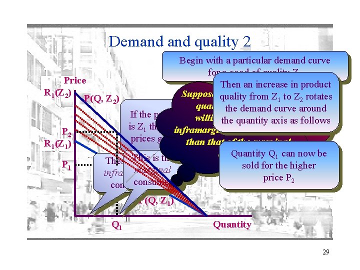
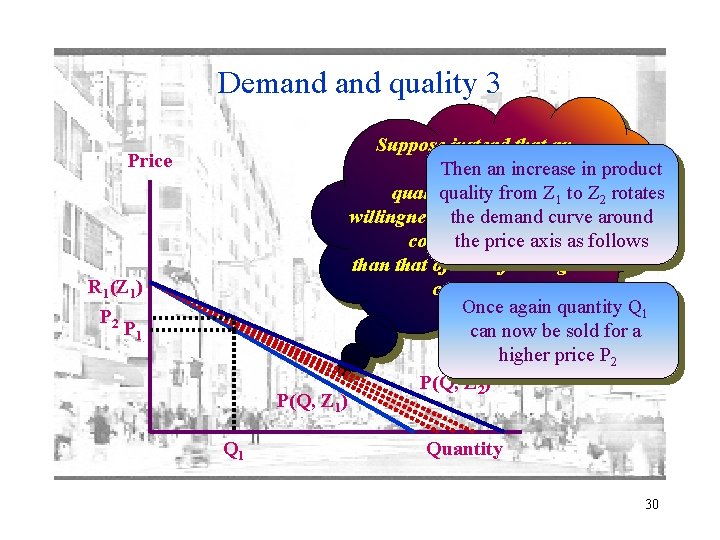
Demand quality • We might think of individual demand as being of the form – Qi = 1 if Pi < Ri(Z) and = 0 otherwise for each consumer i – Each consumer buys exactly one unit so long as price is less than her reservation price – the reservation price is affected by product quality Z • Assume that consumers vary in their reservation prices • Then aggregate demand is of the form P = P(Q, Z) • An increase in product quality increases demand 28

Demand quality 2 Begin with a particular demand curve for a good of quality Z 1 Price Then an increase in product R 1(Z 2) Suppose that an from increase quality Z 1 toin. Z 2 rotates P(Q, Z 2) quality the increases demandthe curve around If the price is P 1 willingness and the product quality to pay of the quantity axis as follows is Z then all consumers with reservation 1 inframarginal consumers more P 2 prices greater than P the good 1 will that of buy the marginal R 1(Z 1) Quantity Q 1 can now be consumer This is the These are the P 1 sold for the higher marginal inframarginal price P 2 consumers P(Q, Z 1) Q 1 Quantity 29

Demand quality 3 Price R 1(Z 1) P 2 P 1 P(Q, Z 1) Q 1 Suppose instead that an Then anin increase in product increase fromthe Z 1 to Z 2 rotates quality increases thepay demand curve around willingness to of marginal the price axis as follows consumers more than that of the inframarginal consumers Once again quantity Q 1 can now be sold for a higher price P 2 P(Q, Z 2) Quantity 30

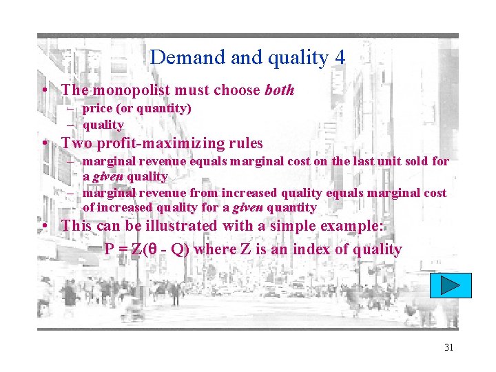
Demand quality 4 • The monopolist must choose both – price (or quantity) – quality • Two profit-maximizing rules – marginal revenue equals marginal cost on the last unit sold for a given quality – marginal revenue from increased quality equals marginal cost of increased quality for a given quantity • This can be illustrated with a simple example: P = Z( - Q) where Z is an index of quality 31

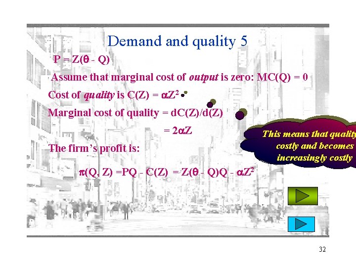
Demand quality 5 P = Z( - Q) Assume that marginal cost of output is zero: MC(Q) = 0 Cost of quality is C(Z) = a. Z 2 Marginal cost of quality = d. C(Z)/d(Z) = 2 a. Z The firm’s profit is: This means that quality costly and becomes increasingly costly p(Q, Z) =PQ - C(Z) = Z( - Q)Q - a. Z 2 32

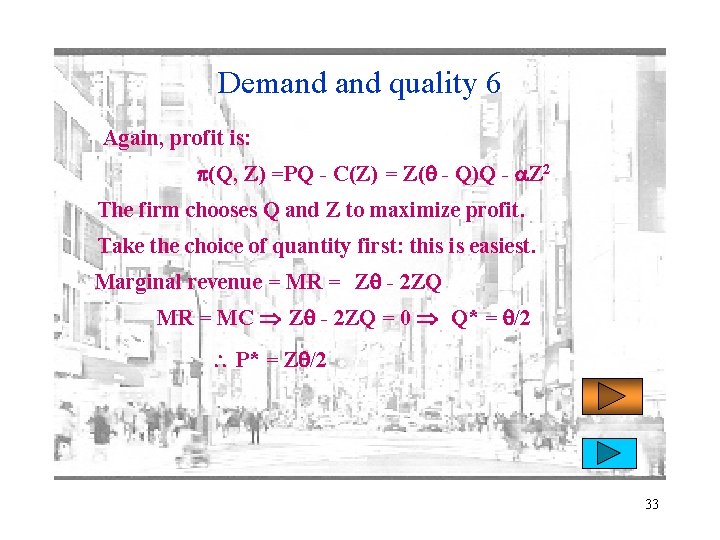
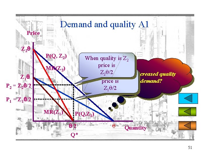
Demand quality 6 Again, profit is: p(Q, Z) =PQ - C(Z) = Z( - Q)Q - a. Z 2 The firm chooses Q and Z to maximize profit. Take the choice of quantity first: this is easiest. Marginal revenue = MR = Z - 2 ZQ MR = MC Z - 2 ZQ = 0 Q* = /2 P* = Z /2 33

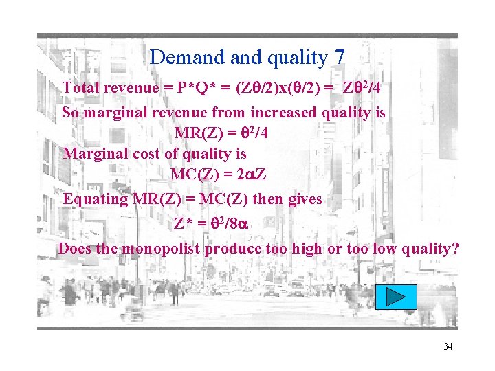
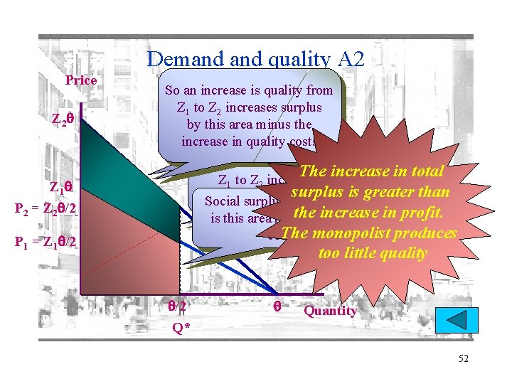
Demand quality 7 Total revenue = P*Q* = (Z /2)x( /2) = Z 2/4 So marginal revenue from increased quality is MR(Z) = 2/4 Marginal cost of quality is MC(Z) = 2 a. Z Equating MR(Z) = MC(Z) then gives Z* = 2/8 a Does the monopolist produce too high or too low quality? 34

Demand quality: multiple products • What if the firm chooses to offer more than one product? – what qualities should be offered? – how should they be priced? • Determined by costs and consumer demand 35

Demand quality: multiple products 2 • An example: – two types of consumer – each buys exactly one unit provided that consumer surplus is nonnegative – if there is a choice, buy the product offering the larger consumer surplus – types of consumer distinguished by willingness to pay for quality • This is vertical product differentiation 36

Vertical differentiation • Indirect utility to a consumer of type i from consuming a product of quality z at price p is Vi = qi(z – zi) – p – where i measures willingness to pay for quality; – zi is the lower bound on quality below which consumer type i will not buy – assume 1 > 2: type 1 consumers value quality more than type 2 – assume z 1 > z 2 = 0: type 1 consumers only buy if quality is greater than z 1: • never fly in coach • never shop in Wal-Mart • only eat in “good” restaurants – type 2 consumers will buy any quality so long as consumer surplus is nonnegative 37

Vertical differentiation 2 • Firm cannot distinguish consumer types • Must implement a strategy that causes consumers to selfselect – persuade type 1 consumers to buy a high quality product z 1 at a high price – and type 2 consumers to buy a low quality product z 2 at a lower price, which equals their maximum willingness to pay • Firm can produce any product in the range z, z • MC = 0 for either quality type 38

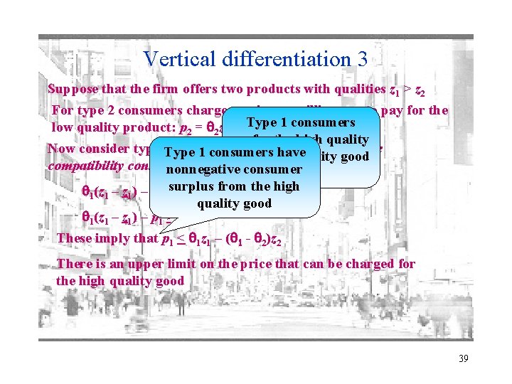
Vertical differentiation 3 Suppose that the firm offers two products with qualities z 1 > z 2 For type 2 consumers charge maximum willingness to pay for the low quality product: p 2 = 2 z 2 Type 1 consumers prefer the high quality Now consider type 1 Type consumers: firm have faces an incentive 1 consumers to the low quality good compatibility constraint nonnegative consumer high 1(z 1 – z 1) – p 1 >surplus 1(z 2 – from z 1) – pthe 2 quality good 1(z 1 – z 1) – p 1 > 0 These imply that p 1 < 1 z 1 – ( 1 - 2)z 2 There is an upper limit on the price that can be charged for the high quality good 39

Vertical differentiation 4 • Take the equation p 1 = 1 z 1 – ( 1 – 2)z 2 – – this is increasing in quality valuations increasing in the difference between z 1 and z 2 quality can be prices highly when it is valued highly firm has an incentive to differentiate the two products’ qualities to soften competition between them • monopolist is competing with itself • What about quality choice? – prices p 1 = 1 z 1 – ( 1 – 2)z 2; p 2 = 2 z 2 • check the incentive compatibility constraints – suppose that there are N 1 type 1 and N 2 type 2 consumers 40

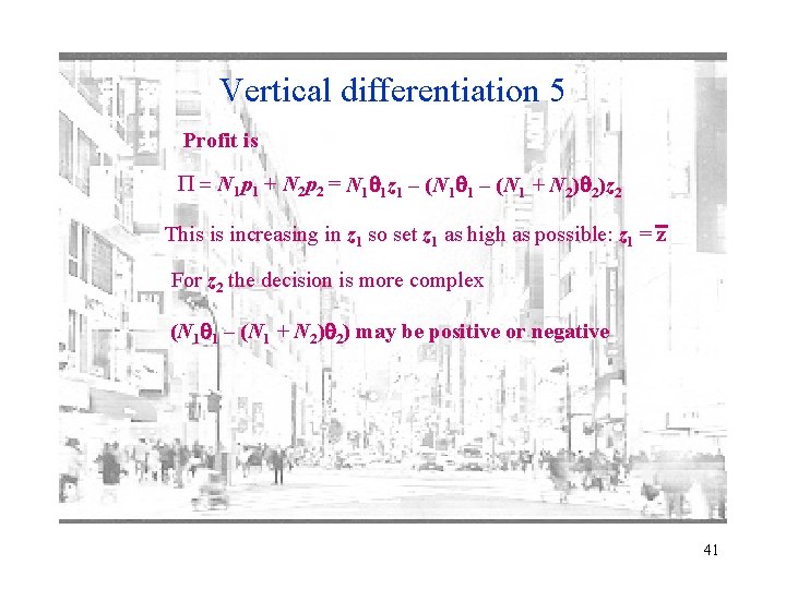
Vertical differentiation 5 Profit is P = N 1 p 1 + N 2 p 2 = N 1 1 z 1 – (N 1 + N 2) 2)z 2 This is increasing in z 1 so set z 1 as high as possible: z 1 = z For z 2 the decision is more complex (N 1 1 – (N 1 + N 2) 2) may be positive or negative 41

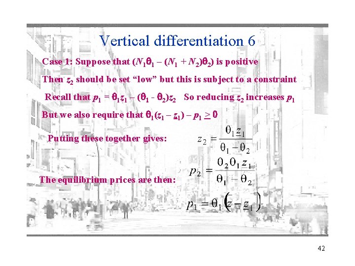
Vertical differentiation 6 Case 1: Suppose that (N 1 1 – (N 1 + N 2) 2) is positive Then z 2 should be set “low” but this is subject to a constraint Recall that p 1 = 1 z 1 – ( 1 - 2)z 2 So reducing z 2 increases p 1 But we also require that 1(z 1 – z 1) – p 1 > 0 Putting these together gives: The equilibrium prices are then: 42

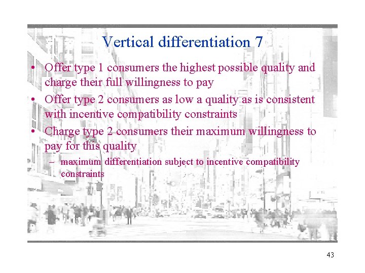
Vertical differentiation 7 • Offer type 1 consumers the highest possible quality and charge their full willingness to pay • Offer type 2 consumers as low a quality as is consistent with incentive compatibility constraints • Charge type 2 consumers their maximum willingness to pay for this quality – maximum differentiation subject to incentive compatibility constraints 43

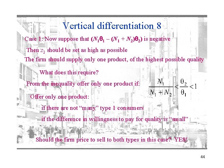
Vertical differentiation 8 Case 1: Now suppose that (N 1 1 – (N 1 + N 2) 2) is negative Then z 2 should be set as high as possible The firm should supply one product, of the highest possible quality What does this require? From the inequality offer only one product if: Offer only one product: if there are not “many” type 1 consumers if the difference in willingness to pay for quality is “small” Should the firm price to sell to both types in this case? YES! 44

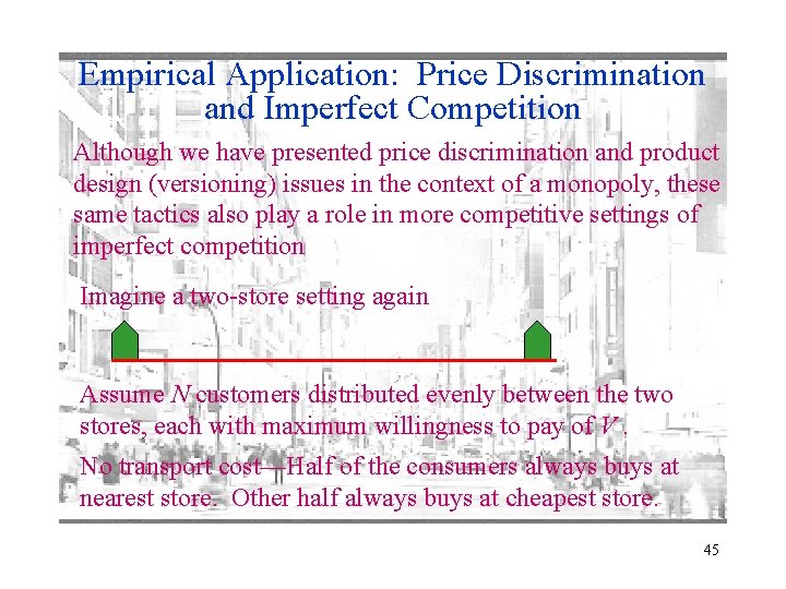
Empirical Application: Price Discrimination and Imperfect Competition Although we have presented price discrimination and product design (versioning) issues in the context of a monopoly, these same tactics also play a role in more competitive settings of imperfect competition Imagine a two-store setting again Assume N customers distributed evenly between the two stores, each with maximum willingness to pay of V. No transport cost—Half of the consumers always buys at nearest store. Other half always buys at cheapest store. 45

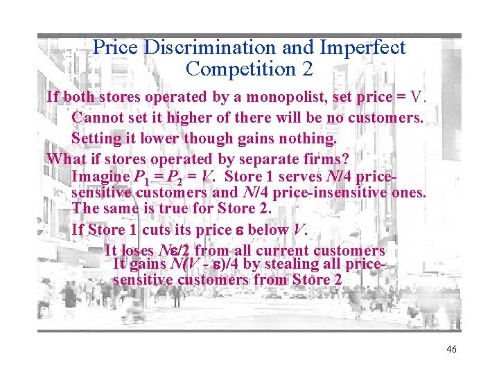
Price Discrimination and Imperfect Competition 2 If both stores operated by a monopolist, set price = V. Cannot set it higher of there will be no customers. Setting it lower though gains nothing. What if stores operated by separate firms? Imagine P 1 = P 2 = V. Store 1 serves N/4 pricesensitive customers and N/4 price-insensitive ones. The same is true for Store 2. If Store 1 cuts its price below V. It loses N /2 from all current customers It gains N(V - )/4 by stealing all pricesensitive customers from Store 2 46

Price Discrimination and Imperfect Competition 3 MORAL 1: Both firms have a real incentive to cut price. This ultimately proves self-defeating In equilibrium, both still serve N/2 customers but now do so at a price closer to cost. This is especially frustrating in light of the “brandloyal” or price-insensitive customers Cutting their price does not increase their likelihood of shopping at a particular place. It just loses revenue. MORAL 2: Unlike the monopolist who sets the same price to everyone, these firms have an incentive to discriminate and so continue to charge a high price to loyal consumers while pricing low to others. 47

Price Discrimination and Imperfect Competition 4 The intuition then is that price discrimination may be associated with imperfect competition and become more prominent as markets get more competitive (but still less than perfectly competitive). This idea is tested by Stavins (2001) with airline prices. Restrictions such as a required Saturday night stay-over or an advanced purchase serve as screening mechanism for price-sensitive customers. Hence, restrictions lead to lower ticket price. Stavins (2001) idea is that price reduction associated with flight restrictions will be small in markets that are not very competitive. 48

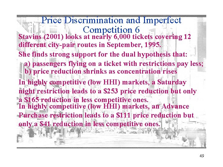
Price Discrimination and Imperfect Competition 6 Stavins (2001) looks at nearly 6, 000 tickets covering 12 different city-pair routes in September, 1995. She finds strong support for the dual hypothesis that: a) passengers flying on a ticket with restrictions pay less; b) price reduction shrinks as concentration rises In highly competitive (low HHI) markets, a Saturday night restriction leads to a $253 price reduction but only a $165 reduction in less competitive ones. In highly competitive (low HHI) markets, an Advance Purchase restriction leads to a $111 price reduction but only a $41 reduction in less competitive ones. 49

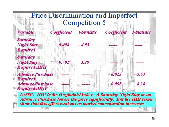
Price Discrimination and Imperfect Competition 5 Variable Saturday Night Stay Requiredx. HHI Coefficient t-Statistic – 0. 408 – 4. 05 ----- 0. 792 3. 39 ----- Advance Purchase ----– 0. 023 – 5. 53 Required Advance Purchase ----0. 098 8. 38 Requiredx. HHI NOTE: HHI is the Herfindahl Index. A Saturday Night Stay or an Advance Purchase lowers the price significantly. But the HHI terms show that this effect weakens as market concentration increases. 50

Demand quality A 1 Price Z 2 P(Q, Z 2) When quality is Z 2 price is 2 q/2 Howisdoes When. Zquality Z 1 increased quality price is affect demand? Z 1 q/2 MR(Z 2) Z 1 P 2 = Z 2 /2 P 1 = Z 1 /2 MR(Z 1) P(Q, Z 1) /2 Q* q Quantity 51

Demand quality A 2 Price Z 2 Z 1 P 2 = Z 2 /2 P 1 = Z 1 /2 So an increase is quality from Z 1 to Z surplus 2 increases Social surplus at quality Z 2 area minus the is by this area minus quality increase in quality costs An increase in quality from The increase in total Z 1 to Z 2 increases surplus revenue by this area Zis greater than Social surplus at quality 1 the increase in profit. is this area minus quality The monopolist produces costs too little quality /2 Q* Quantity 52

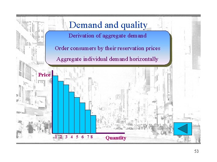
Demand quality Derivation of aggregate demand Order consumers by their reservation prices Aggregate individual demand horizontally Price 1 2 3 4 5 6 78 Quantity 53

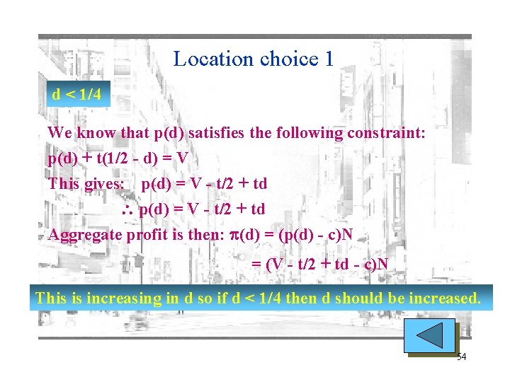
Location choice 1 d < 1/4 We know that p(d) satisfies the following constraint: p(d) + t(1/2 - d) = V This gives: p(d) = V - t/2 + td Aggregate profit is then: p(d) = (p(d) - c)N = (V - t/2 + td - c)N This is increasing in d so if d < 1/4 then d should be increased. 54

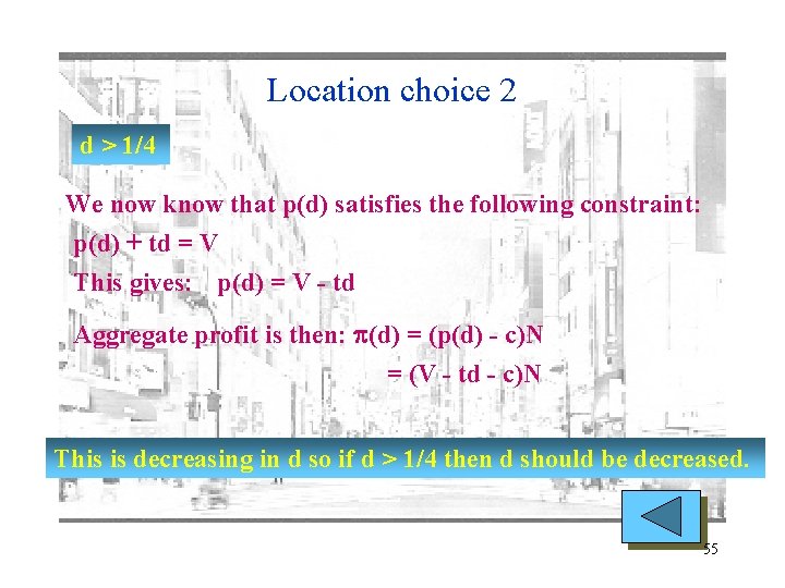
Location choice 2 d > 1/4 We now know that p(d) satisfies the following constraint: p(d) + td = V This gives: p(d) = V - td Aggregate profit is then: p(d) = (p(d) - c)N = (V - td - c)N This is decreasing in d so if d > 1/4 then d should be decreased. 55

Commodity Bundling and Tie-In Sales 56

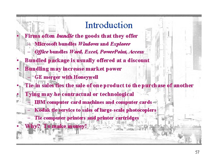
Introduction • Firms often bundle the goods that they offer – Microsoft bundles Windows and Explorer – Office bundles Word, Excel, Power. Point, Access • Bundled package is usually offered at a discount • Bundling may increase market power – GE merger with Honeywell • Tie-in sales ties the sale of one product to the purchase of another • Tying may be contractual or technological – IBM computer card machines and computer cards – Kodak tie service to sales of large-scale photocopiers – Tie computer printers and printer cartridges • Why? To make money! 57

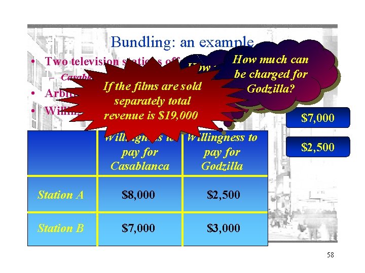
Bundling: an example How much canfilms • Two television stations offered two old Hollywood How much can be charged for – Casablanca and Son of Godzilla be charged for If the films are sold Godzilla? • Arbitrage is possible between. Casablanca? the stations separately total • Willingnessrevenue to pay is: is $19, 000 $7, 000 Willingness to pay for Casablanca Godzilla Station A $8, 000 $2, 500 Station B $7, 000 $3, 000 $2, 500 58

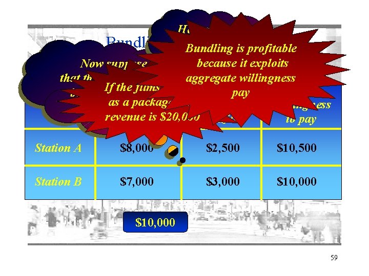
Bundling: How much can an example 2 be. Bundling charged forprofitable is thebecause package? it exploits Now suppose aggregate willingness that the two films are If and the films Willingness to sold Willingness Total payto bundled sold are as pay a package total pay for Willingness as a package revenue is $20, 000 Godzilla Casablanca to pay Station A $8, 000 $2, 500 $10, 500 Station B $7, 000 $3, 000 $10, 000 59

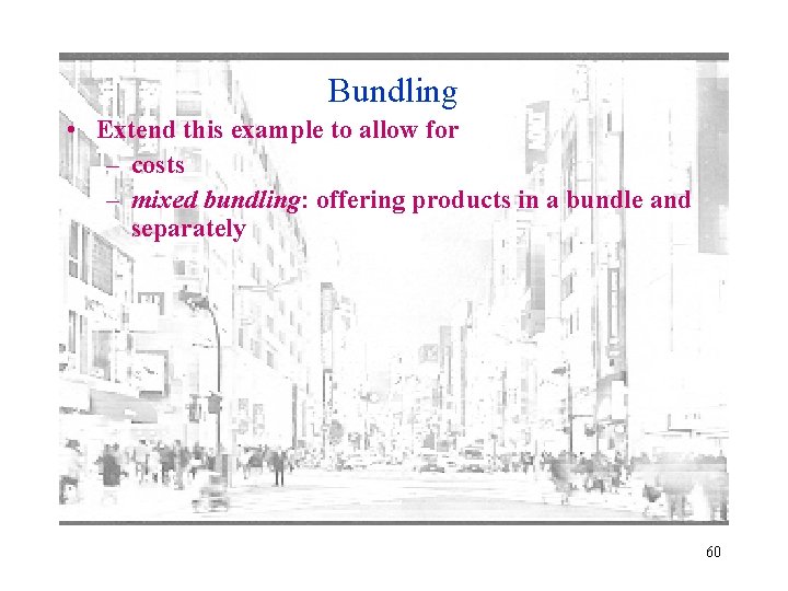
Bundling • Extend this example to allow for – costs – mixed bundling: offering products in a bundle and separately 60

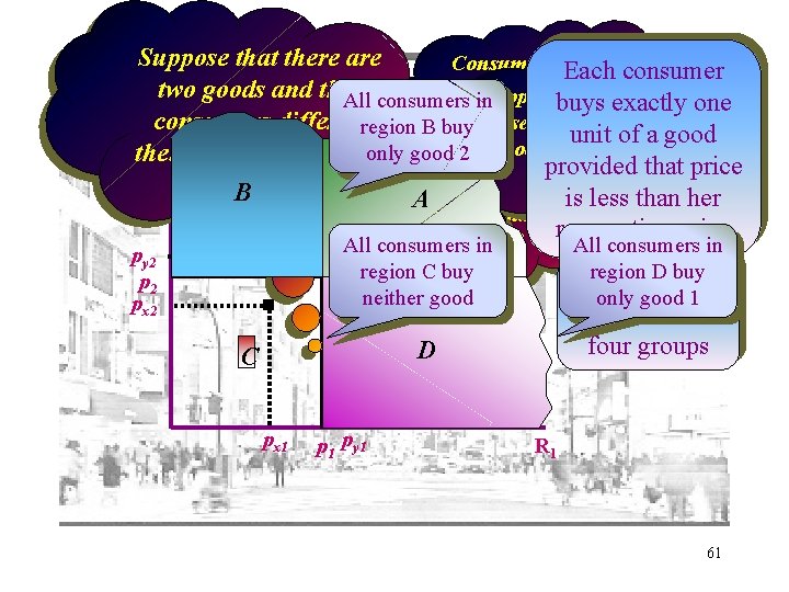
Suppose that there are Consumer y Each has consumer reservation price two goods and that Bundling: another thatpy 1 the firm one All consumersexample in. Supposebuys exactly for goodsets 1 and py 2 p for in All consumers price consumers differ inregion B buy 1 unit of abuy good for good 2 region A good 1 and price p R only Consumer good 2 2 their reservation prices 2 x hasprovided that both 2 goods price for good for these reservation price px 1 is less than her B goods A for good 1 and px 2 for good 2 reservation price y py 2 px 2 x All consumers in region C buy neither good All consumers in region D buy Consumers only good 1 split into four groups D C px 1 py 1 R 1 61

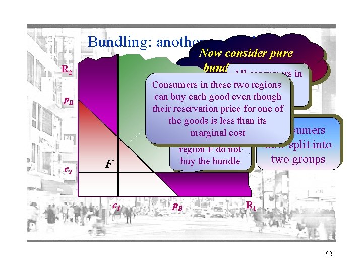
Bundling: another example 2 Now consider pure bundling at some All consumers in p. B E buy Consumers in theseprice two regions region R 2 can buy each good eventhe though bundle their reservation price for one of Ethe goods is less than its Consumers cost All marginal consumers in p. B c 2 F c 1 now split into two groups region F do not buy the bundle p. B R 1 62

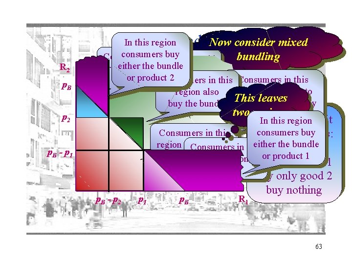
Mixed bundling R 2 p. B p 2 p. B - p 1 In this region Now consider mixed consumers buy Consumers in Good this bundling 1 is sold either theonly bundle region buy at price p 1 or product 2 in this good 2 Consumers in. Good this 2 Consumers is sold region are willing to region also at price p 2 This leaves both goods. They buy the bundle buy two regions buy the bundle Consumers In this regionsplit consumers buy Consumers in this into four groups: either the bundle region buy nothing in this Consumers The bundle is sold buy the bundle or product 1 region at price p. Bbuy < p 1 only + pbuy only good 1 2 good 1 p. B - p 2 p 1 p. B R 1 buy only good 2 buy nothing 63

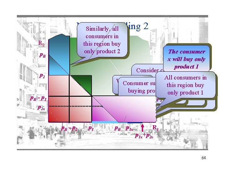
Mixed bundling 2 Similarly, all consumers in this region buy only product 2 R 2 The consumer x will buy only product 1 Consider consumer x with consumers reservation. All prices p 1 x for in Which is this Consumer surplus from Consumer surplus region from buy product 1 this and p 2 x for measure Her aggregate willingness buying product 1 isbundle the only is 1 product 2 product to pay for the bundle is p 1 x -pp 1 + p - p 1 x 2 x+ p 2 x. B x p. B p 2 p. B - p 1 p 2 x p. B - p 2 p 1 p. B p 1 x R 1 p 1 x+p 2 x 64

Mixed bundling 3 • What should a firm actually do? • There is no simple answer – mixed bundling is generally better than pure bundling – but bundling is not always the best strategy • Each case needs to be worked out on its merits 65

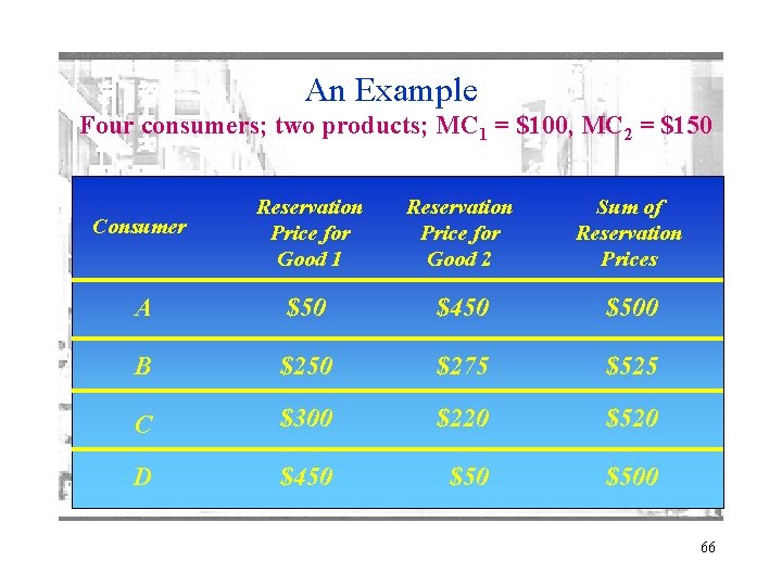
An Example Four consumers; two products; MC 1 = $100, MC 2 = $150 Consumer Reservation Price for Good 1 Reservation Price for Good 2 Sum of Reservation Prices A $50 $450 $500 B $250 $275 $525 C $300 $220 $520 D $450 $500 66

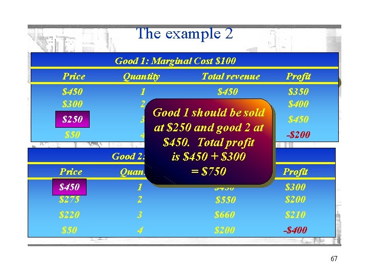
The example 2 Good 1: Marginal Cost $100 Price $450 $300 $250 $50 Price $450 $275 $220 $50 Quantity Total. Consider revenue simple Profit monopoly pricing 1 $450 $350 2 $400 $600 Good 1 should be sold 3 $750 $450 at $250 and good 2 at 4 $200 -$200 $450. Total profit Good 2: Marginal Cost + $150 is $450 $300 Quantity =Total $750 revenue 1 2 3 4 $450 $550 $660 $200 Profit $300 $210 -$400 67

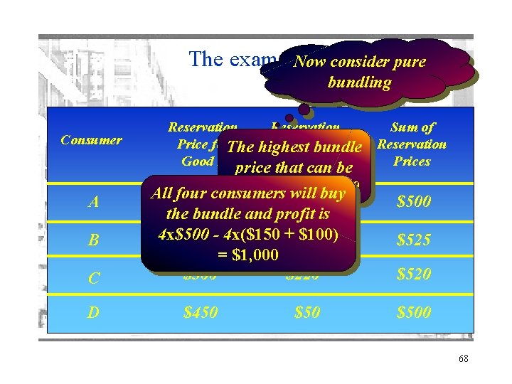
The example 3 consider pure Now bundling Consumer A B C D Reservation Price for. The highest Price for bundle Good 1 price that Good 2 be can considered isbuy $500 All four consumers will $50 $450 the bundle and profit is 4 x$500 $100) $250 - 4 x($150 + $275 = $1, 000 $300 $220 $450 $50 Sum of Reservation Prices $500 $525 $520 $500 68

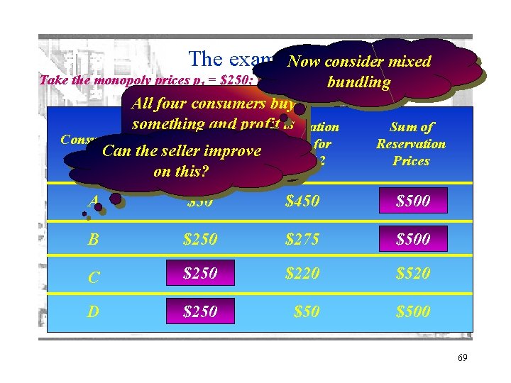
The example Now 4 consider mixed Take the monopoly prices p 1 = $250; p 2 = $450 and a bundle price p. B = $500 bundling All four consumers buy something and profit is Reservation Consumer Price + for$150 x 2 Price for Can the$250 x 2 seller improve Good 1 Good 2 = $800 on this? Sum of Reservation Prices A $50 $450 $500 B $250 $275 $525 $500 C $300 $250 $220 $520 D $450 $250 $500 69

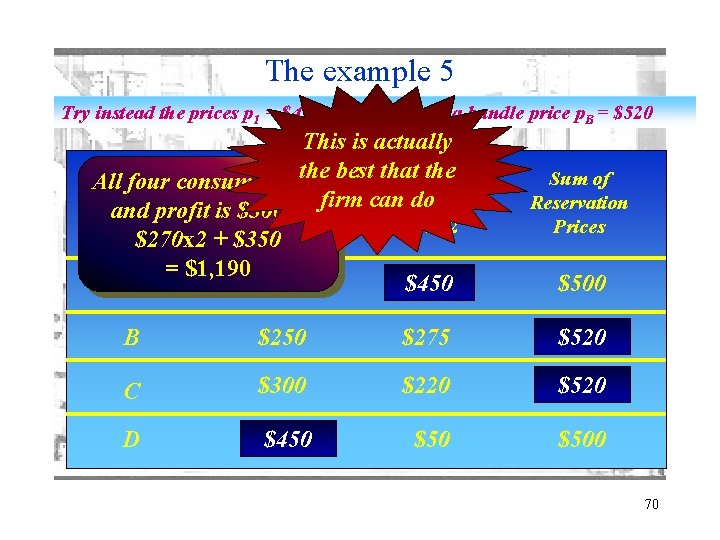
The example 5 Try instead the prices p 1 = $450; p 2 = $450 and a bundle price p. B = $520 This is actually the best Reservation that the Reservation All four consumers buy Consumer do for Price+forfirm can Price and profit is $300 Good 1 $270 x 2 + $350 = $1, 190 A $50 Good 2 Sum of Reservation Prices $450 $500 B $250 $275 $520 C $300 $220 $520 D $450 $500 70

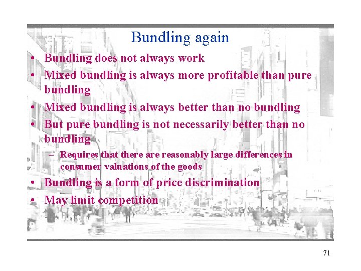
Bundling again • Bundling does not always work • Mixed bundling is always more profitable than pure bundling • Mixed bundling is always better than no bundling • But pure bundling is not necessarily better than no bundling – Requires that there are reasonably large differences in consumer valuations of the goods • Bundling is a form of price discrimination • May limit competition 71

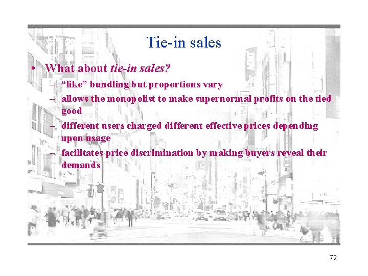
Tie-in sales • What about tie-in sales? – “like” bundling but proportions vary – allows the monopolist to make supernormal profits on the tied good – different users charged different effective prices depending upon usage – facilitates price discrimination by making buyers reveal their demands 72

Tie-in sales 2 • Suppose that a firm offers a specialized product – a camera – that uses highly specialized film cartridges • Then it has effectively tied the sales of film cartridges to the purchase of the camera – this is actually what has happened with computer printers and ink cartridges • How should it price the camera and film? – suppose also that there are two types of consumer, highdemand low-demand, with one-thousand of each type – high demand P = 16 – Qh; low demand P = 12 - Ql – the company does not know which type is which 73

Tie-in sales 3 • Film is produced competitively at $2 per picture – so film is priced at $2 per picture • Suppose that the company leases its cameras – if priced so that all consumers lease then we can ignore production costs of the camera • these are fixed at 2000 c • Now consider the lease terms 74

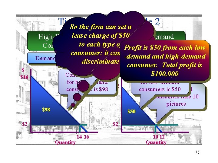
Tie-in sales: an example 2 So the firm can set a $ $16 Recall theof $50 lease that charge High-Demand Low-Demand film sells at $2 Consumers to each type of Profit Consumers is $50 from each low per picture consumer: it cannot High-demand high-demand Demand: P = 16 - Q Demand: and P = 12 -Q discriminate consumers take 14 consumer. Total profit is pictures$ $100, 000 Consumer surplus for high-demand $12 consumers is $98 for low-demand consumers Low-demand is $50 consumers take 10 pictures $50 $2 $2 Quantity 14 16 10 12 Quantity 75

Tie-in sales example 3 • This is okay but there may be room for improvement • Redesign the camera to tie the camera and the film – technological change that makes the camera work only with the firm’s film cartridge • Suppose that the firm can produce film at a cost of $2 per picture • Implement a tying strategy that makes it impossible to use the camera without this film 76

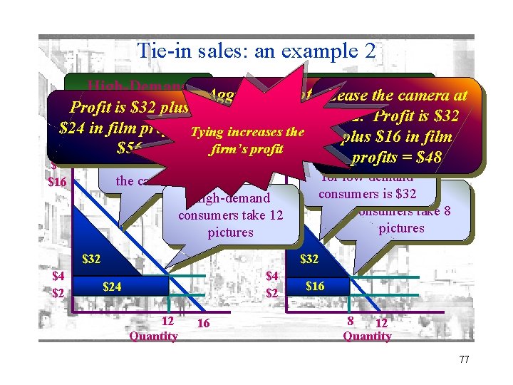
Tie-in sales: an example 2 High-Demand Aggregate profit Low-Demand is now the camera at Lease Profit is $32 plus Consumers $48, 000 + $56, 000 = Profit is $32. $24 in film profits Tying = increases the. Demand: $104, 000 plus. P =$16 Demand: P = 16 - Q 12 -in. Qfilm Each firm’s profit $56 high-demand profits = $48 Consumer surplus consumer will lease $ $ the camera at $32 High-demand $12 consumers take 12 pictures $16 $32 $4 $2 for low-demand consumers Low-demand is $32 consumers take 8 pictures $32 $4 $2 $24 12 Quantity 16 $16 8 12 Quantity 77

Tie-in sales example 3 • Why does tying increase profits? – high-demand consumers are offered a quantity discount under both the original and the tied lease arrangement – but tying solves the identification and arbitrage problems • film exploits monopoly in film supply • high-demand consumers are revealed by their film purchases • quantity discount is then used to increase profit • arbitrage is not an issue: both types of consumers pay the same lease and the same unit price for film 78

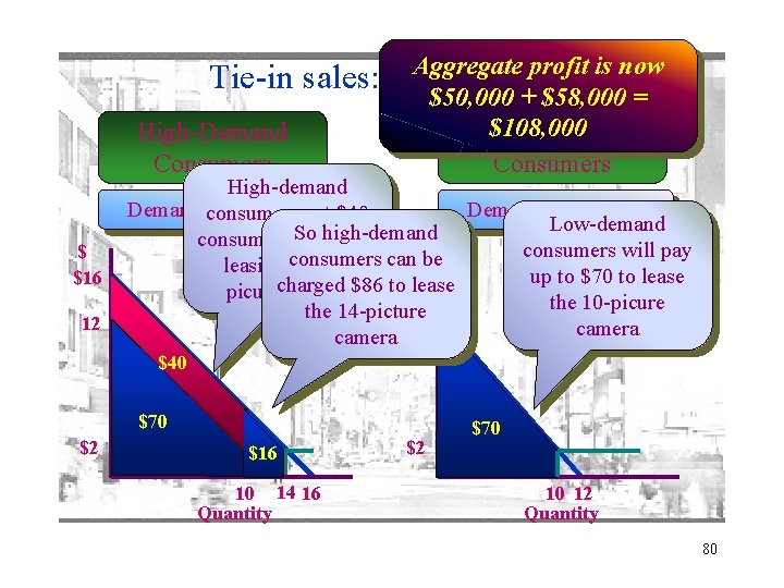
Tie-in sales example 4 • Can the firm do even better? • Redesign the camera so that the film cartridge is integral – offer two types of integrated camera/film package: high capacity and low capacity – what capacities? • This is similar to second-degree price discrimination – design two cameras with socially efficient capacities: 10 picture and 14 picture – lease these as integrated packages 79

Tie-in sales: High-Demand Consumers $ $16 12 Aggregate profit is now an $50, 000 example 2 + $58, 000 = $108, 000 Low-Demand Consumers High-demand Demand: consumers P = 16 - Q get $40 Demand: P = 12 - Q Low-demand So high-demand consumer surplus by consumers will pay can$ be leasing consumers the 10 up to $70 to lease picurecharged camera $86 to lease the 10 -picure $12 the 14 -picture camera $40 $70 $2 $16 10 14 16 Quantity $2 $70 10 12 Quantity 80

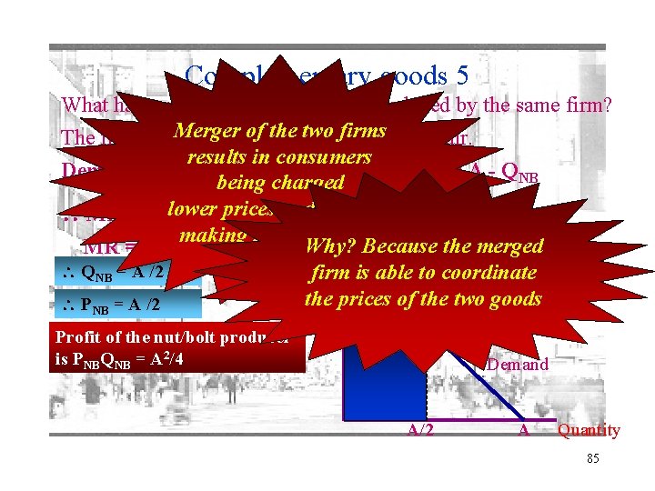
Complementary goods • Complementary goods are goods that are consumed together – nuts and bolts – PC monitors and computer processors • How should these goods be produced? • How should they be priced? • Take the example of nuts and bolts – these are perfect complements: need one of each! • Assume that demand for nut/bolt pairs is: Q = A - (PB + PN) 81

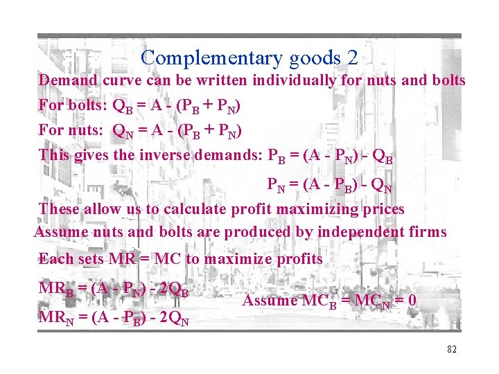
Complementary goods 2 Demand curve can be written individually for nuts and bolts For bolts: QB = A - (PB + PN) For nuts: QN = A - (PB + PN) This gives the inverse demands: PB = (A - PN) - QB PN = (A - PB) - QN These allow us to calculate profit maximizing prices Assume nuts and bolts are produced by independent firms Each sets MR = MC to maximize profits MRB = (A - PN) - 2 QB MRN = (A - PB) - 2 QN Assume MCB = MCN = 0 82

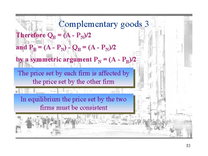
Complementary goods 3 Therefore QB = (A - PN)/2 and PB = (A - PN) - QB = (A - PN)/2 by a symmetric argument PN = (A - PB)/2 The price set by each firm is affected by the price set by the other firm In equilibrium the price set by the two firms must be consistent 83

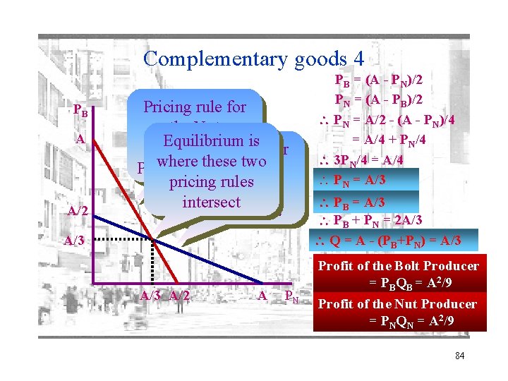
Complementary goods 4 PB A A/2 Pricing rule for the Nut Equilibrium is for Producer: Pricing rule two PN where = (A - these Pthe )/2 Bolt B pricing rules Producer: Pintersect B = (A - PN)/2 A/3 A/2 A PN PB = (A - PN)/2 PN = (A - PB)/2 PN = A/2 - (A - PN)/4 = A/4 + PN/4 3 PN/4 = A/4 PN = A/3 PB + PN = 2 A/3 Q = A - (PB+PN) = A/3 Profit of the Bolt Producer = PBQB = A 2/9 Profit of the Nut Producer = PNQN = A 2/9 84

Complementary goods 5 What happens if the two goods are produced by the same firm? of the The firm will. Merger set a price PNBtwo forfirms a nut/bolt pair. results in consumers Demand is now QNB = A - PNB so that PNB = A - QNB being charged $ lower prices and the firm MRNB = A - 2 QNB making greater profits Why? MR = MC = 0 A Because the merged QNB = A /2 firm is able to coordinate the prices of the two goods PNB = A /2 Profit of the nut/bolt producer is PNBQNB = A 2/4 A/2 Demand MR A/2 A Quantity 85

Complementary goods 6 • Don’t necessarily need a merger to get these benefits – product network • ATM networks • airline booking systems – one of the markets is competitive • price equals marginal cost in this market • leads to the “merger” outcome • There may also be a countervailing force – network externalities • value of a good to consumers increases when more consumers use the good 86

Network externalities • Product complementarities can generate network effects – Windows and software applications • substantial economies of scale • strong network effects – leads to an applications barrier to entry • new operating system will sell only if applications are written for it • but… • So product complementarities can lead to monopoly power being extended 87

Anti-trust and bundling • The Microsoft case is central – accusation that used power in operating system (OS) to gain control of browser market by bundling browser into the OS – need to show • monopoly power in OS • OS and browser are separate products with no need to be bundled • abuse of power to maintain or extend monopoly position – Microsoft argued that technology required integration – further argued that it was not “acting badly” • consumers would benefit from lower price because of the complementarity between OS and browser 88

Microsoft and Netscape • Complementarity products – – so merge? what if Netscape refuses? then Microsoft can develop its own browser MC ≈ 0 so competition in the browser market drives price close to zero – but then get the outcome of merger firm through competition • So Microsoft is not “acting badly” • But – JAVA allows applications to be run on Internet browsers – Netscape then constitutes a threat – need to reduce their market share 89

And now… • This view gained more force & support in Europe – bundling of Media Player into Windows – Competition Directorate found against Microsoft • Microsoft Appealed • Microsoft finally lost its appeal in September, 2007 – Result: Microsoft ordered to stop bundling and forced to pay fine of € 497 (finally settled in October, 2007) – Some economists upset by this decision arguing that as price discrimination, bundling often expands the market, AND also that bundling/tying can reflect competition and not just market power 90

Competitive Bundling/Tying • Bundling and tying are very commonly observed phenomena – Perhaps too commonly observed to be just the outcome of monopoly power – Is there a way to understand competitive bundling? • Yes! Salinger and Evans (2005) and Evans (2006) • It may well be the case that the structure of demand the nature of scope and scale economies force competitive firms to bundle tie their goods 91

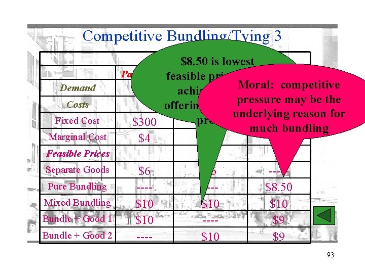
Competitive Bundling/Tying 2 • Consider the table on the next slide and assume consumer willingness to pay is $20 for most preferred option – Competitive firm can’t offer pain reliever & decongestant separately, To do so incurs • total fixed cost of $600 • Marginal cost of $4 • Breakeven price = $6 – 50 by pain relief alone and pay $6 per unit – 50 by decongestant alone and pay $6 per unit – 100 buy both and pay $12 per combined unit • Total Revenue = $1800; Total cost = $600 + $4 x 150 = $1800 – Rival could sell bundled product for $10 and steal all 100 customers interested in joint goods who now pay $12 92

Competitive Bundling/Tying 3 Demand Costs Fixed Cost Marginal Cost Product $8. 50 is lowest Pain Relieffeasible Decongestant price and is. Bundle Moral: 100 competitive 50 by only achieve pressure may be the offering the bundled underlying reason for product $300 much bundling $4 $4 $7 50 Feasible Prices Separate Goods Pure Bundling Mixed Bundling Bundle + Good 1 Bundle + Good 2 $6 ---$10 ----$8. 50 $10 $9 $9 93

Antitrust and tying arrangements • Tying arrangements have been the subject of extensive litigation • Current policy – tie-in violates antitrust laws if • there exists distinct products: tying product & tied one • firm tying the products has sufficient market power in the tying market to force purchase of the tied good • tying arrangement forecloses or has the potential to foreclose a substantial volume of trade • As time passes, approach is more and more of a rule-ofreason standard with increasing recognition that whether price discrimination or competitive pressure is the reason, bundling/tying is often welfare-improving 94