6 MONOPOLY Contents monopoly characteristics causes of monopoly

6. MONOPOLY

Contents • • monopoly characteristics causes of monopoly existence monopoly equilibrium Lerner index monopoly supply curve price discrimination productive and allocative efficiency monopoly regulation

Monopoly characteristics • monopoly IS a type of competition (competition accross the market) • existence of SOLE subject on the supply side • restricted entry • monopoly is a „price maker“ • no close substitutes to the monopoly´s production • individual demand curve = market demand curve

Causes of monopoly existence – increasing returns to scale – decreasing AC: • sole firm is able to satisfy the entire market demand more effectively than in case of many firms in the industry • cause: relatively high fixed costs (mostly infrastructure) to the individual demand NATURAL MONOPOLY typically network industries (water-supply, sewer systems etc. )

Natural monopoly • ≠ natural resources monopoly • eventual demonopolization would lead to the monopoly anyway. . . because: • each firm would attend relatively low demand upon high costs • typical: minimum of AC lies above the individual demand curve • usually highly profitable industry → motivation to enter the industry → investments into research → technological progress → costs decrease → dismantling the entry barriers (i. e. telecommunication)

Natural monopoly – endeavour to demonopolization CZK/Q firm upon non-monopoly situation. . . CZK/Q . . . rise of monopoly AC AC d=AR Q Upon non-monopoly conditions a specific firm cannot exist – AC always higher than AR, due to relatively low market share D=AR Q Monopoly as a natural result – the sole firm is able to attend more effectively the market demand

Causes of monopoly existence – natural resources monopoly • the sole firm controls (owns) all natural resources needed to produce the specific good • example: . . . ? ? ?

Causes of monopoly existence – artificial monopoly State intervention: • state grants an exclusive right to produce a specific good to the only firm, or: • state founds a monopoly firm in a specific industry • i. e. : Czech Post (missive delivery), Central banks (banknotes and coins emission) Copyrights, patents

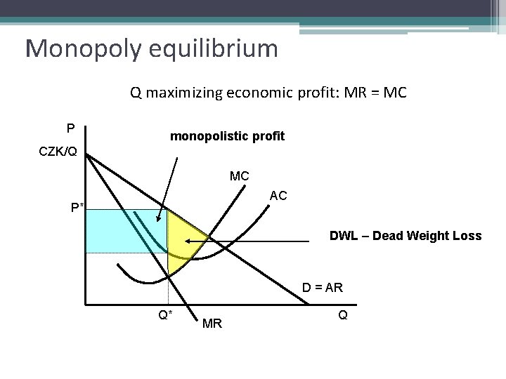
Monopoly equilibrium Q maximizing economic profit: MR = MC P monopolistic profit CZK/Q MC AC P* DWL – Dead Weight Loss D = AR Q* MR Q

Monopolistic profit • monopoly is able to gain a profit either in long run (entry restrictions) • volume of profit/loss depends on the individual demand firm´s costs • if monopoly gains loss, the crucial criterion is the same as for the perfect competition firm (it also has to cover its VC in SR, or TC in LR)

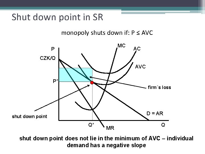
Shut down point in SR monopoly shuts down if: P ≤ AVC MC P AC CZK/Q AVC P* firm´s loss D = AR shut down point Q* MR Q shut down point does not lie in the minimum of AVC – individual demand has a negative slope

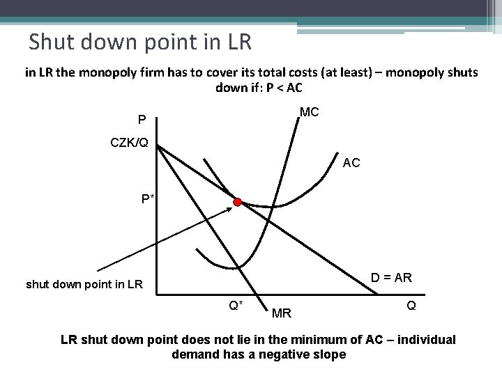
Shut down point in LR the monopoly firm has to cover its total costs (at least) – monopoly shuts down if: P < AC MC P CZK/Q AC P* D = AR shut down point in LR Q* MR Q LR shut down point does not lie in the minimum of AC – individual demand has a negative slope

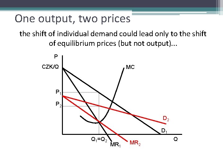
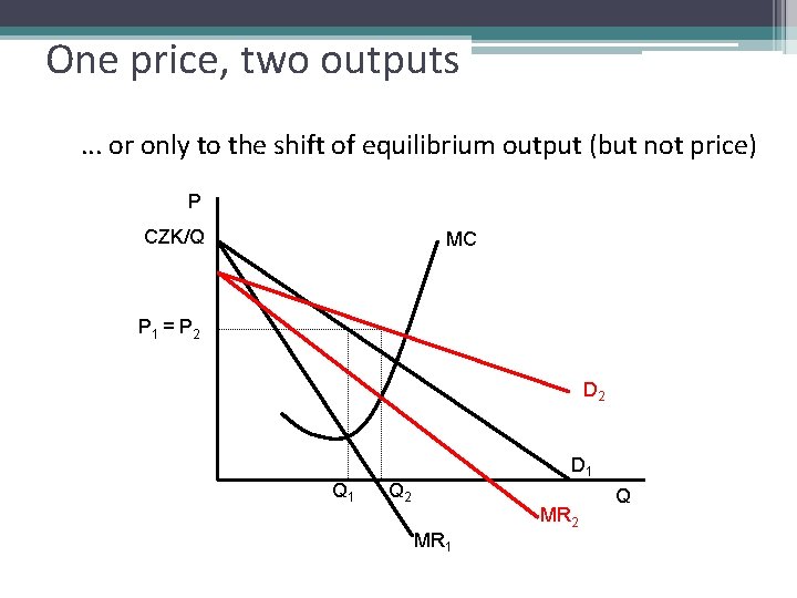
Monopoly supply curve is not possible to derive, because: • spots of equilibria do not lie on the MC function • we cannot acquire any set of spots which would represent a certain relationship between equilibrium price and output • moreover – if the firm´s demand shifts: there could be one equilibrium output for several equilibrium prices, or one equilibrium price for several equilibirum outputs

One output, two prices the shift of individual demand could lead only to the shift of equilibrium prices (but not output). . . P CZK/Q MC P 1 P 2 D 1 Q 1=Q 2 MR 1 MR 2 Q

One price, two outputs. . . or only to the shift of equilibrium output (but not price) P CZK/Q MC P 1 = P 2 D 2 Q 1 D 1 Q 2 MR 1 MR 2 Q

Multivalent relationship between equilibrium output and price P CZK/Q MC Monopoly supply curve? ? ? D 2 D 3 D 1 Q 3 Q 2 MR 1 MR 3 MR 2 Q

Setting the monopoly price • monopoly cannot set its equilibrium price wherever it wants → must respect its individual demand • equilibrium price lies above the monopoly MC • the difference between MC and equilibrium price is determined by the price elasticity of demand • the less elastic demand the higher difference between P and MC

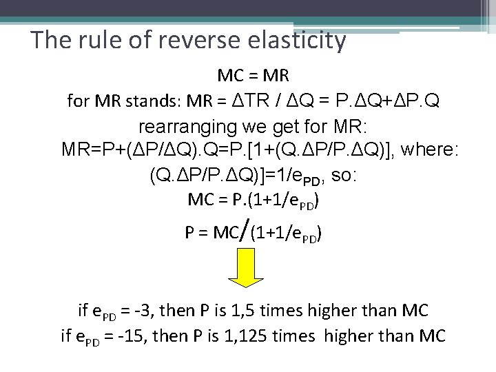
The rule of reverse elasticity MC = MR for MR stands: MR = ΔTR / ΔQ = P. ΔQ+ΔP. Q rearranging we get for MR: MR=P+(ΔP/ΔQ). Q=P. [1+(Q. ΔP/P. ΔQ)], where: (Q. ΔP/P. ΔQ)]=1/e. PD, so: MC = P. (1+1/e. PD) P = MC/(1+1/e. PD) if e. PD = -3, then P is 1, 5 times higher than MC if e. PD = -15, then P is 1, 125 times higher than MC

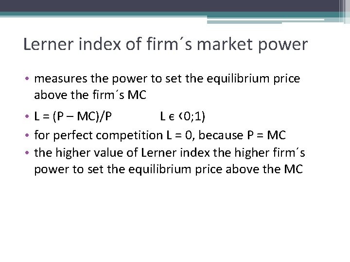
Lerner index of firm´s market power • measures the power to set the equilibrium price above the firm´s MC • L = (P – MC)/P L є ‹ 0; 1) • for perfect competition L = 0, because P = MC • the higher value of Lerner index the higher firm´s power to set the equilibrium price above the MC

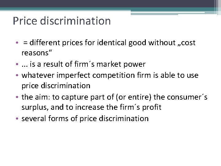
Price discrimination • = different prices for identical good without „cost reasons“ • . . . is a result of firm´s market power • whatever imperfect competition firm is able to use price discrimination • the aim: to capture part of (or entire) the consumer´s surplus, and to increase the firm´s profit • several forms of price discrimination

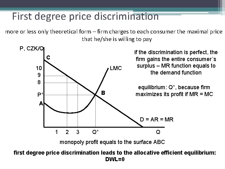
First degree price discrimination more or less only theoretical form – firm charges to each consumer the maximal price that he/she is willing to pay P, CZK/Q C 10 9 8 LMC B P* if the discrimination is perfect, the firm gains the entire consumer´s surplus – MR function equals to the demand function equilibrium: Q*, because firm maximizes its profit if MR = MC A D = AR = MR 1 2 3 Q* Q monopoly profit equals to the surface ABC first degree price discrimination leads to the allocative efficient equilibrium: DWL=0

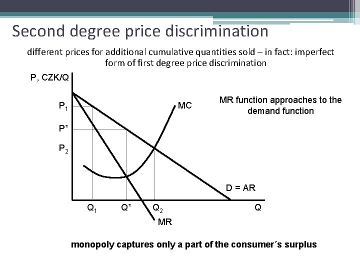
Second degree price discrimination different prices for additional cumulative quantities sold – in fact: imperfect form of first degree price discrimination P, CZK/Q P 1 MC MR function approaches to the demand function P* P 2 D = AR Q 1 Q* Q 2 Q MR monopoly captures only a part of the consumer´s surplus

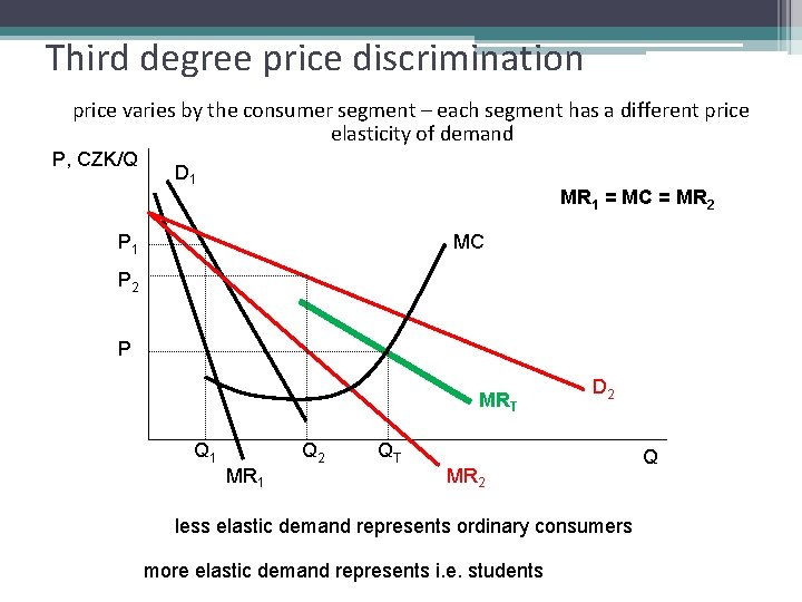
Third degree price discrimination price varies by the consumer segment – each segment has a different price elasticity of demand P, CZK/Q D 1 MR 1 = MC = MR 2 P 1 MC P 2 P MRT Q 1 MR 1 Q 2 QT D 2 MR 2 less elastic demand represents ordinary consumers more elastic demand represents i. e. students Q

Third degree price discrimination Works if: • firm is able to divide the entire demand by a specific attribute to different segments - price elasticity • consumers are disallowed to trade the goods among each other (i. e. registered flight tickets) or. . . • . . . transaction costs too high to be effective to trade the goods among consumers (i. e. shipping costs) – compare prices of brand goods in USA and Europe

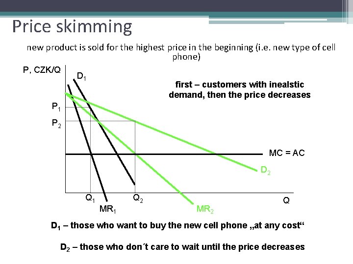
Price skimming new product is sold for the highest price in the beginning (i. e. new type of cell phone) P, CZK/Q D 1 first – customers with inealstic demand, then the price decreases P 1 P 2 MC = AC D 2 Q 1 MR 1 Q 2 MR 2 Q D 1 – those who want to buy the new cell phone „at any cost“ D 2 – those who don´t care to wait until the price decreases

Price skimming Prices of selected models of cell phones (Sept. 2007 – May 2008) Samsung E 210 Source: www. mobilmania. cz Sony Ericsson K 550 i 8 ay /0 08 r/ /0 8 M Nokia 5300 XM Ap ar Fe Ja Motorola KRZR K 1 M 08 b/ 08 n/ 07 c/ LG KG 800 Chocolate De 7 /0 No v 7 /0 Oc t Se p/ 07 7000 6500 6000 5500 5000 4500 4000 3500 3000

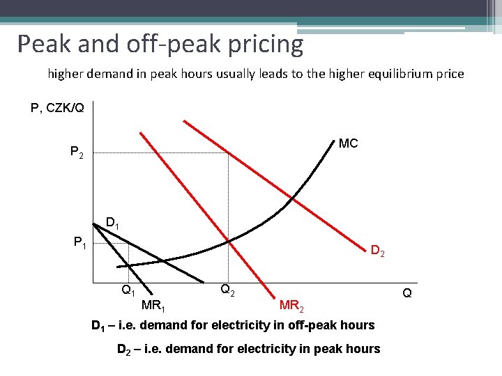
Peak and off-peak pricing higher demand in peak hours usually leads to the higher equilibrium price P, CZK/Q MC P 2 D 1 P 1 D 2 Q 1 MR 1 Q 2 MR 2 D 1 – i. e. demand for electricity in off-peak hours D 2 – i. e. demand for electricity in peak hours Q

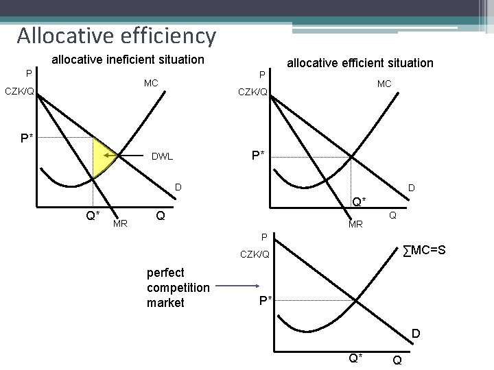
Allocative and productive efficiency of monopoly • monopoly is allocative and productive inefficient • Allocative efficiency – existence of DWL – part of the consumers´ and producer´s surplus is lost – less quantity for higher price than upon perfect competition conditions • Productive efficiency – monopoly does not minimize its AC on equilibrium output (neither in SR nor in LR)

Allocative efficiency allocative ineficient situation P P MC CZK/Q allocative efficient situation MC CZK/Q P* P* DWL D D Q* Q* MR Q P ∑MC=S CZK/Q perfect competition market P* D Q* Q

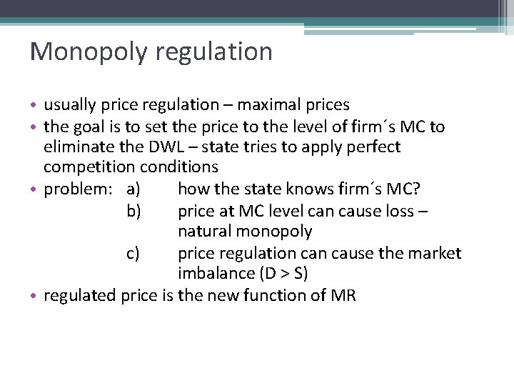
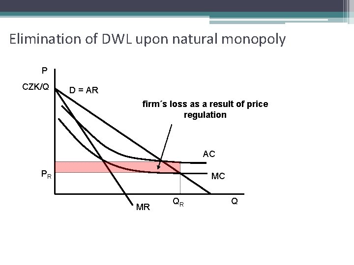
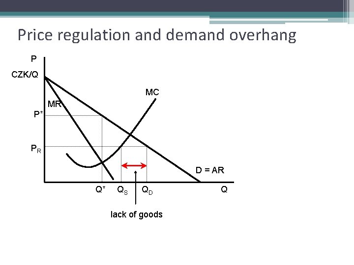
Monopoly regulation • usually price regulation – maximal prices • the goal is to set the price to the level of firm´s MC to eliminate the DWL – state tries to apply perfect competition conditions • problem: a) how the state knows firm´s MC? b) price at MC level can cause loss – natural monopoly c) price regulation cause the market imbalance (D > S) • regulated price is the new function of MR

Elimination of DWL upon natural monopoly P CZK/Q D = AR firm´s loss as a result of price regulation AC PR MC MR QR Q

Price regulation and demand overhang P CZK/Q MC MR P* PR D = AR Q* QS QD lack of goods Q