Potential Outcomes Group Treatment group D 1 Control

 Control group (D")
")

 Control group (D = 0)")


, Propensity Score Analysis. Thousand")


 V (unobserved) A F G U (unobserved)")


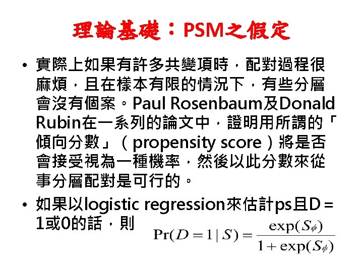
建議是 |Pi – Pj| < ε, 而")

,ATU(average treatment effect on the untreated")
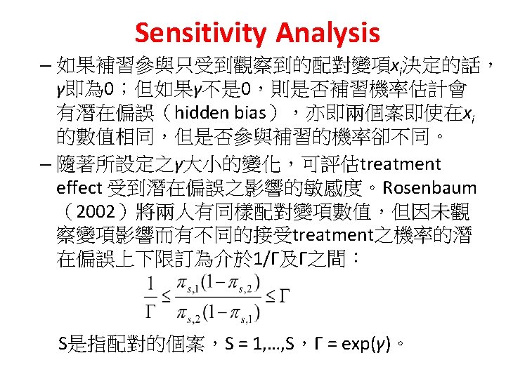
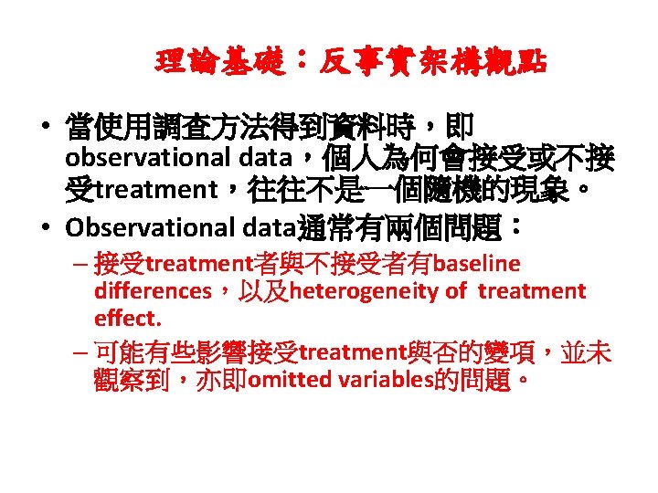
的資料cattaneo 2( http: //www. stata. com/manuals 13/te. pdf )。 •")


")
")
")


")


. 58778666")
")
 using “teffects (psmatch)”")
 using “teffects (psmatch)”")
 等 – SPSS: SPSS Macro")


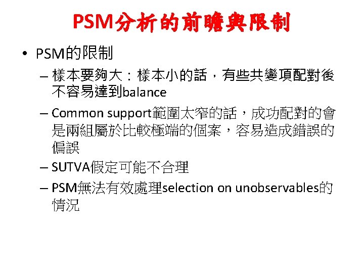
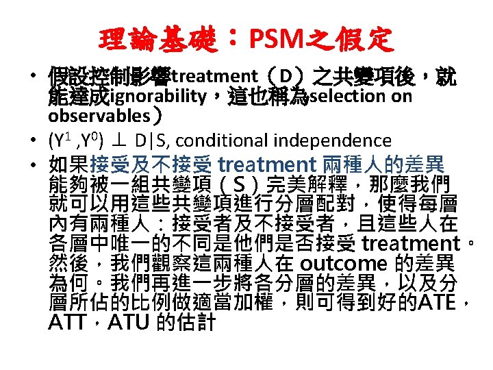
 • Selection on unobservables")


- Slides: 62
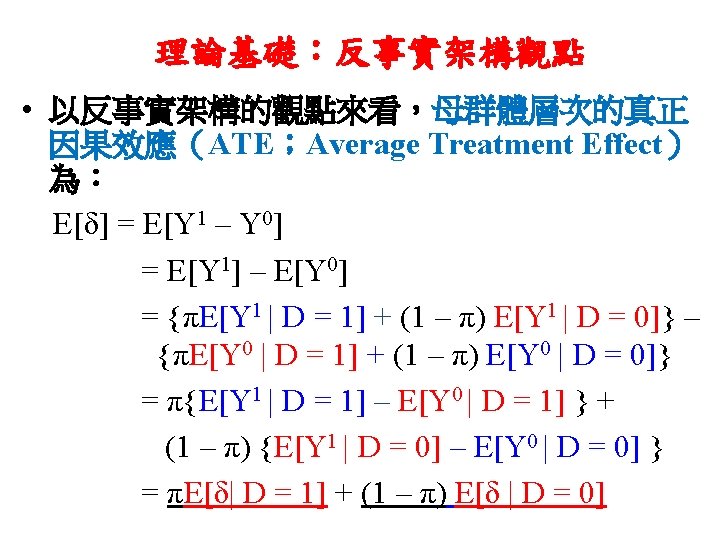
理論基礎 • 反事實架構觀點的因果推論想像 Potential Outcomes Group Treatment group (D = 1) Control group (D = 0) Y 1 Y 0 Observable Counterfactual Observable
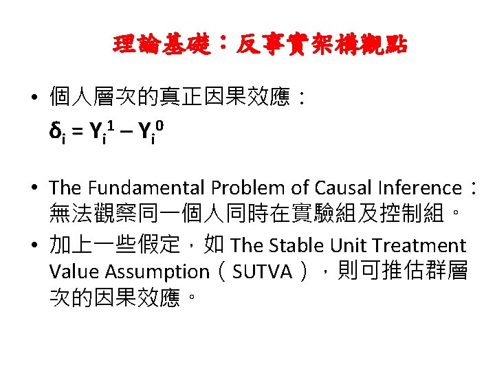
理論基礎 S D Confounding variables δ W Y (causal effect of interest)
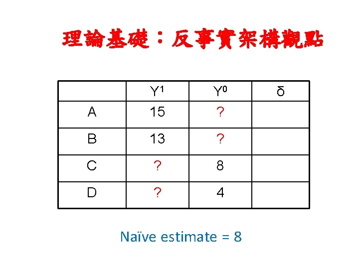
理論基礎:反事實架構觀點 Potential Outcomes Group Treatment group (D = 1) Control group (D = 0) Y 1 Y 0 Observable E[Y 1 | D = 1] Counterfactual Observable E[Y 1 | D = 0] E[Y 0 | D = 1]
理論基礎:反事實架構觀點 A Y 1 15 Y 0 10 δ 5 B 13 8 5 C 13 8 5 D 9 4 5 ATT = ATU; ATE = 5
理論基礎:反事實架構觀點 A Y 1 15 Y 0 10 δ 5 B 13 8 5 C 11 8 3 D 7 4 3 ATT ≠ ATU; ATE = 4
理論基礎:反事實架構觀點 Naïve Estimate = average causal effect + baseline bias + differential effect bias E[Y 1 |D = 1] – E[Y 0|D = 0] = E(δ) + {E(Y 0|D=1) − E(Y 0|D=0)} +{E(δ |D=1) − E(δ |D=0)} (1−π)
理論基礎:Why PSM? • Guo, Shenyang & Mark W. Fraser (2010), Propensity Score Analysis. Thousand Oaks, CA: Sage. • Monte Carlo simulation study of Chapter 8; mean of 10, 000 samples • Selection on observable simulation (p. 288 -296) – Model: y = 100 +. 5 x 1 +. 2 x 2 -. 5 x 3 +. 5 W + u W* =. 5 Z +. 1 x 3 + v – Estimation • OLS regerssion: 0. 5375; Bias= 0. 375 (7. 5% over) • PSM: 0. 4875; Bias= -0. 0125 (2. 5% under)
理論基礎:Why PSM? A model of selection on observables
PSM OLS Models relationship between confounders and treatment Models relationship between confounders and outcome No routine assumptions about linearity and interactions Generally assumes linearity and absence of interaction, but this can be relaxed Easy assessment of overlap – Overlap is assessed in multilittle potential for extrapolation dimensional space – often extrapolated Causal effect for treated, untreated, local comparison Sample size can be diminished through matching, loss of power Causal effect extrapolated to population Sample size stays constant, power can increase due to covariates
PSM 分析之步驟 Selection • Selection of covariates that may affect the assignment of the treatment (D=1 or 0) Estimation • Estimate propensity scores using either logistic regression or other means Matching Model Checks Effect Estimation Sensitivity Analysis • Choose matching algorithm • Check covariates balance • Check the region of common support • Mean difference • Standard error • Check if the estimated result is robust against hidden bias
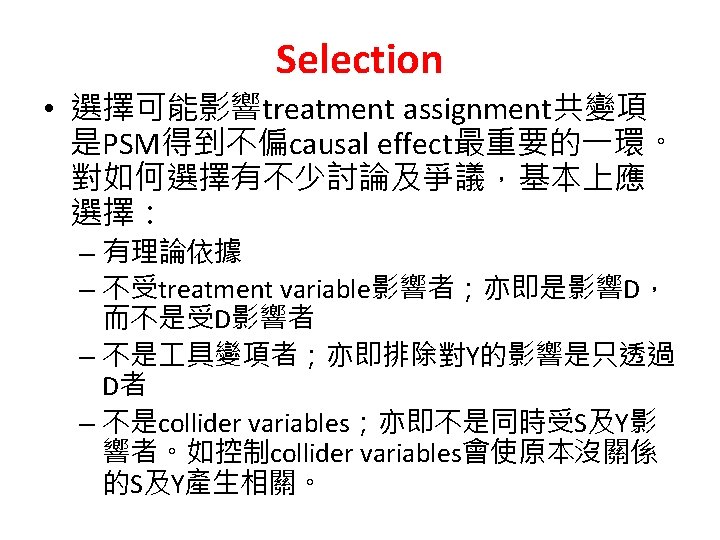
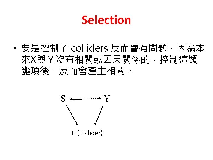
Selection: Which covariates should be controlled A B C F G D Y
Selection (控制 B & F 即可,Why? ) V (unobserved) A F G U (unobserved) B C D Y
Estimation • 通常可用logistic regression或probit regression來估計ps。 • 也有用data mining 或 optimization 的方法, 及尋找最大解釋力的模型,如generalized boosted regression (如Stata之boost程式)。
Matching • 從事PSM的運算方法可歸成以下大類: – Nearest Neighbor Matching: 1: 1 或 1:k – Optimal Matching: 1: 1 或 1:k – Full Matching: k – Interval Matching – Kernel Matching – 不同運算方法的差異: • With or without replacement • How many units to match
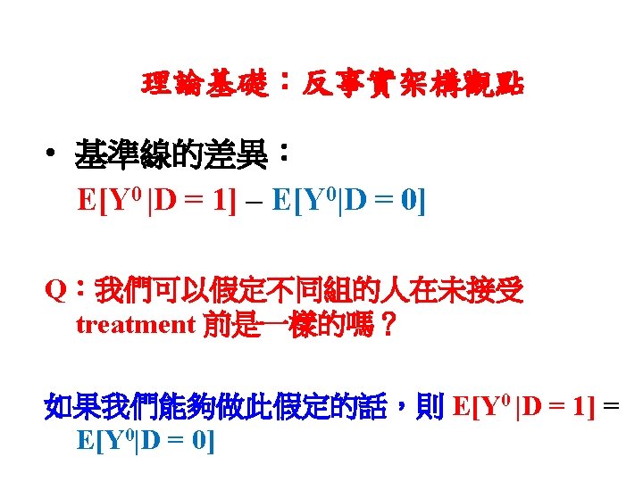
Matching • Caliper及trimming之考量 – Caliper:界定可配對之ps間的合理距離, Rosenbaum & Rubin(1985)建議是 |Pi – Pj| < ε, 而 ε ≦. 25 σp , σp 為 estimated ps的 標準差。 – Trimming: 界定common support之範圍,排除 treatment cases所配對之non-treated cases的ps density 是低於某個比例(如2%、5%或 10%) 時,因 ps 分配的兩端可能是極端的個案。
Model Checks • Check the region of common support:通常 可以圖形如histogram,來檢視兩組之ps分 配重疊的情況。
Effect Estimation • PSM可估計ATT(average treatment effect on the treated),ATU(average treatment effect on the untreated )及ATE(average treatment effect,如果所有的人都接受treatmet的話)。通 常感興趣的是ATT,因為我們期待如果接受 treatment者會有效果。可以進一步分成推論到配 對樣本(如SATT)及母群體的treatment effects( PATT)。 • 如何估計psm所得到之estimates的standard errors有不同的看法。不同的matching會有不同估 計se的方法,其中一種是用bootstrapping方式求 得PSM估計值的se(但有爭議)。
PSM:實例演練 • 以Stata 13介紹新指令teffects(treatment effect)的資料cattaneo 2( http: //www. stata. com/manuals 13/te. pdf )。 • Treatment: mbsmoke; Outcome: bweight • Covariates: mmarried, mage, prenatal 1, fbaby • 程式: – psmatch 2: user written, Stata 13及以下均可 用 – teffects psmatch: Stata 13
PSM:實例演練 Naïve Estimate
PSM:實例演練 OLS regression with covariates
PSM:實例演練 PSM: 1 to 1 nearest neighbor (ATT, ATU, ATE)
PSM:實例演練 PSM: 1 to 1 nearest neighbor (ATT, ATU, ATE)
PSM:實例演練 PSM: 1 to 1 nearest neighbor (ATT only)
PSM:實例演練 PSM: balance check
PSM:實例演練 Using boosted regression to estimate ps
PSM:實例演練 PSM: 1 to 1 nearest neighbor with ps estimated by boosted regresion (ATT only)
PSM:實例演練 PSM: balance check (once again)
PSM:實例演練 Fitted versus actual values for logistic regression and boosting on the test data set
PSM:實例演練 PSM: check common support using “psgraph”
PSM:實例演練 PSM: using bootstrapping to estimate the standard error of ATT
PSM:實例演練 PSM: sensitivity analysis . disp log(1. 8). 58778666
PSM:實例演練 • PSM: 1 to 5 within caliper (. 25*σps)
PSM:實例演練 • PSM: 1 to 5 within caliper (. 25*σps) using “teffects (psmatch)”
PSM:實例演練 • PSM: 1 to 5 within caliper (. 25*σps) using “teffects (psmatch)”
PSM:實例演練 • 可從事PSM的軟體及程式: – Stata: psmatch 2、nnmatch、teffects (v. 13) 等 – SPSS: SPSS Macro for Propensity Score Matching (http: //ssw. unc. edu/VRC/Lectures/index. htm) – SAS: “GREEDY” Macro (http: //www 2. sas. com/proceedings/sugi 26/proceed. pdf) – R: “Match. It”, “Matching”等 • 另見 Software for implementing matching methods and propensity scores • “http: //www. biostat. jhsph. edu/~estuart/propensityscore software. html”
PSM分析的前瞻與限制 • PSM可用來分析 – 或兩個以上treatments:應用multinomial logistic 或 ordered logistic regression來估計ps – Binary outcome:估計odds ratio,relative risks, risk differences等 • PS與其他分析方法的結合: – Stratification:將estimated ps分層檢視不同分層 的treatment effects – Weighting:利用ps來建構權數,以平衡不同的 群體 – Regression adjustment:將ps視為共變項
PSM分析的前瞻與限制 • PSM與其他分析方法的結合 – 與迴歸分析結合 – 應用在multilevel analysis – 應用在complex sampling – Mediation analysis:從counterfactual framework的角度來看,mediation(也就是 瞭解causal mechanisms)的分析是頗複雜的, 因為中介變項本身就是一種outcome,也就需 要瞭解 counterfactual 的狀態。 – Sequential matching – 其他:如 fixed effects 或 random effects models
PSM分析的前瞻與限制 • selection on unobservables Z D Y U (unobservable) • Selection on unobservables 情況需要用其他適 當的資料(如長期追蹤)及分析方法(如 fixed effects)
PSM入門參考文獻 • Morgan, Stephen L. , and Christopher Winship. 2007. Counterfactuals and Causal Analysis: Methods and Principles for Social Research. Cambridge, MA: Harvard University Press. • Caliendo, Marco, and Sabine Kopeinig. 2008. “Some Practical Guidance for the Implementation of Propensity Score Matching. ” Journal of Economic Surveys 22 (1): 31– 72. • Guo, Shenyang, and Mark. W. Fraser. 2010. Propensity Score Analysis: Statistical Methods and Applications. Los Angeles: Sage.