Physics Analysis Concepts with Panda Root 3 PANDA

Physics Analysis Concepts with Panda. Root (3) PANDA Lecture Week 2017 GSI, Dec 11 - 15, 2017 Klaus Götzen GSI Darmstadt

Topics • Effective Analysis - Working with ROOT TTrees • Event Generators: Evt. Gen, DPM, FTF, Box Generator • Generation and Simulation – Stand-alone generation (simple. Evt. Gen, DPMGen, FTFGen) – Fast Simulation (Pnd. Fast. Sim, Pnd. Fsm. . . ) K. Götzen PANDA Lecture Week 2017 - GSI 2

EFFECTIVE ANALYSIS ROOT TREES

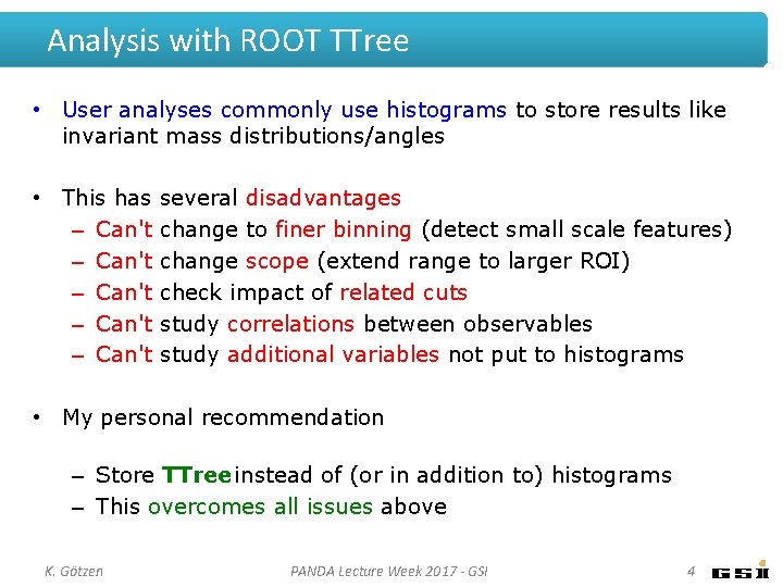
Analysis with ROOT TTree • User analyses commonly use histograms to store results like invariant mass distributions/angles • This has – Can't – Can't several disadvantages change to finer binning (detect small scale features) change scope (extend range to larger ROI) check impact of related cuts study correlations between observables study additional variables not put to histograms • My personal recommendation – Store TTree instead of (or in addition to) histograms – This overcomes all issues above K. Götzen PANDA Lecture Week 2017 - GSI 4

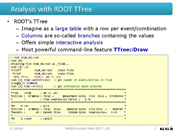
Analysis with ROOT TTree • ROOT's TTree – Imagine as a large table with a row per event/combination – Columns are so-called branches containing the values – Offers simple interactive analysis – Most powerful command-line feature TTree: : Draw > root ntp 0_dd. root [0] Attaching file ntp 0_dd. root as _file 0. . . root [1]. ls TFile** ntp 0_dd. root chain files TFile* ntp 0_dd. root chain files KEY: TTree ntp 0; 1 D 0 ->K- pi+ root [2] ntp 0 ->Get. Entries() // get number of events/entries in TTree (Long 64_t) 1710036 root [3] ntp 0 ->Print() // get information about branches *************************************** *Tree : ntp 0 : D 0 ->K- pi+ * *Entries : 1710036 : Total = 1006429833 bytes File Size = 573205551 * * : : Tree compression factor = 1. 76 * *************************************** *Br 0 : ev/I * *Entries : 1710036 : Total Size= 6846211 bytes File Size = 1994787 * *Baskets : 65 : Basket Size= 391168 bytes Compression= 3. 43 * *. . . . . * *Br 1 : cand/I *. . . K. Götzen PANDA Lecture Week 2017 - GSI 5

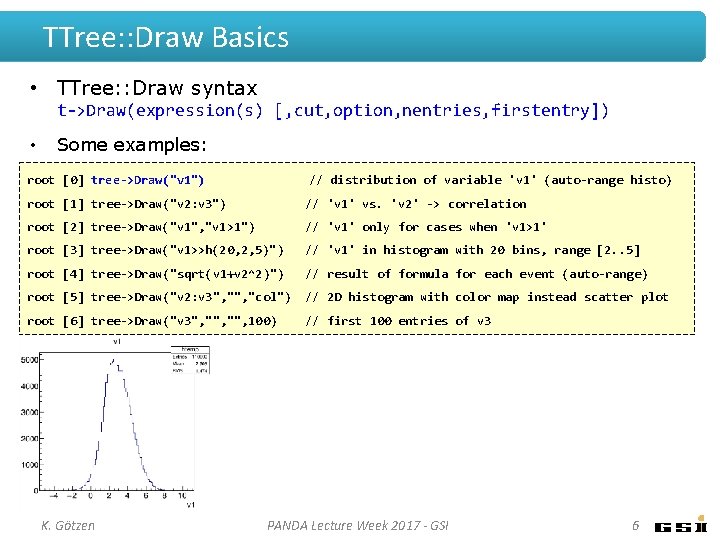
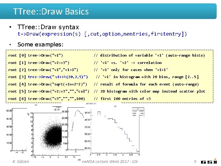
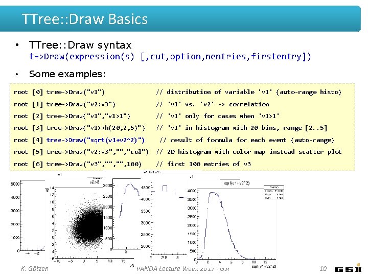
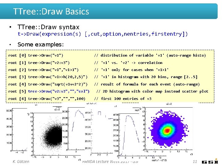
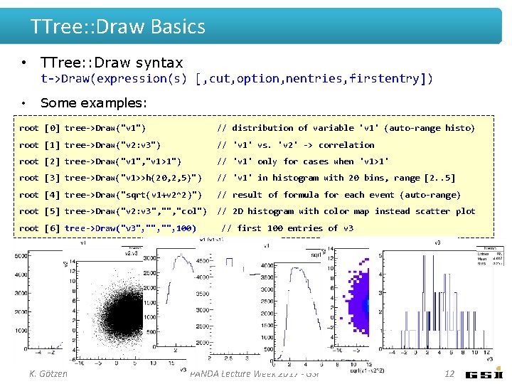
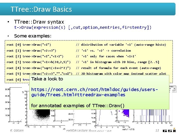
TTree: : Draw Basics • TTree: : Draw syntax t->Draw(expression(s) [, cut, option, nentries, firstentry]) • Some examples: root [0] tree->Draw("v 1") // distribution of variable 'v 1' (auto-range histo) root [1] tree->Draw("v 2: v 3") // 'v 1' vs. 'v 2' -> correlation root [2] tree->Draw("v 1", "v 1>1") // 'v 1' only for cases when 'v 1>1' root [3] tree->Draw("v 1>>h(20, 2, 5)") // 'v 1' in histogram with 20 bins, range [2. . 5] root [4] tree->Draw("sqrt(v 1+v 2^2)") // result of formula for each event (auto-range) root [5] tree->Draw("v 2: v 3", "col") // 2 D histogram with color map instead scatter plot root [6] tree->Draw("v 3", "", 100) // first 100 entries of v 3 K. Götzen PANDA Lecture Week 2017 - GSI 6

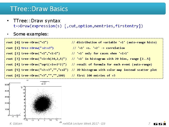
TTree: : Draw Basics • TTree: : Draw syntax t->Draw(expression(s) [, cut, option, nentries, firstentry]) • Some examples: root [0] tree->Draw("v 1") // distribution of variable 'v 1' (auto-range histo) root [1] tree->Draw(" v 2: v 3") // 'v 1' vs. 'v 2' -> correlation root [2] tree->Draw("v 1", "v 1>1") // 'v 1' only for cases when 'v 1>1' root [3] tree->Draw("v 1>>h(20, 2, 5)") // 'v 1' in histogram with 20 bins, range [2. . 5] root [4] tree->Draw("sqrt(v 1+v 2^2)") // result of formula for each event (auto-range) root [5] tree->Draw("v 2: v 3", "col") // 2 D histogram with color map instead scatter plot root [6] tree->Draw("v 3", "", 100) // first 100 entries of v 3 K. Götzen PANDA Lecture Week 2017 - GSI 7

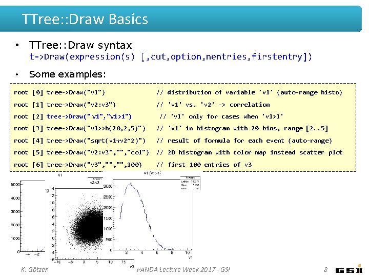
TTree: : Draw Basics • TTree: : Draw syntax t->Draw(expression(s) [, cut, option, nentries, firstentry]) • Some examples: root [0] tree->Draw("v 1") // distribution of variable 'v 1' (auto-range histo) root [1] tree->Draw("v 2: v 3") // 'v 1' vs. 'v 2' -> correlation root [2] tree->Draw(" v 1", "v 1>1") // 'v 1' only for cases when 'v 1>1' root [3] tree->Draw("v 1>>h(20, 2, 5)") // 'v 1' in histogram with 20 bins, range [2. . 5] root [4] tree->Draw("sqrt(v 1+v 2^2)") // result of formula for each event (auto-range) root [5] tree->Draw("v 2: v 3", "col") // 2 D histogram with color map instead scatter plot root [6] tree->Draw("v 3", "", 100) // first 100 entries of v 3 K. Götzen PANDA Lecture Week 2017 - GSI 8

TTree: : Draw Basics • TTree: : Draw syntax t->Draw(expression(s) [, cut, option, nentries, firstentry]) • Some examples: root [0] tree->Draw("v 1") // distribution of variable 'v 1' (auto-range histo) root [1] tree->Draw("v 2: v 3") // 'v 1' vs. 'v 2' -> correlation root [2] tree->Draw("v 1", "v 1>1") // 'v 1' only for cases when 'v 1>1' root [3] tree->Draw(" v 1>>h(20, 2, 5)") // 'v 1' in histogram with 20 bins, range [2. . 5] root [4] tree->Draw("sqrt(v 1+v 2^2)") // result of formula for each event (auto-range) root [5] tree->Draw("v 2: v 3", "col") // 2 D histogram with color map instead scatter plot root [6] tree->Draw("v 3", "", 100) // first 100 entries of v 3 K. Götzen PANDA Lecture Week 2017 - GSI 9

TTree: : Draw Basics • TTree: : Draw syntax t->Draw(expression(s) [, cut, option, nentries, firstentry]) • Some examples: root [0] tree->Draw("v 1") // distribution of variable 'v 1' (auto-range histo) root [1] tree->Draw("v 2: v 3") // 'v 1' vs. 'v 2' -> correlation root [2] tree->Draw("v 1", "v 1>1") // 'v 1' only for cases when 'v 1>1' root [3] tree->Draw("v 1>>h(20, 2, 5)") // 'v 1' in histogram with 20 bins, range [2. . 5] root [4] tree->Draw("sqrt(v 1+v 2^2)") // result of formula for each event (auto-range) root [5] tree->Draw("v 2: v 3", "col") // 2 D histogram with color map instead scatter plot root [6] tree->Draw("v 3", "", 100) // first 100 entries of v 3 K. Götzen PANDA Lecture Week 2017 - GSI 10

TTree: : Draw Basics • TTree: : Draw syntax t->Draw(expression(s) [, cut, option, nentries, firstentry]) • Some examples: root [0] tree->Draw("v 1") // distribution of variable 'v 1' (auto-range histo) root [1] tree->Draw("v 2: v 3") // 'v 1' vs. 'v 2' -> correlation root [2] tree->Draw("v 1", "v 1>1") // 'v 1' only for cases when 'v 1>1' root [3] tree->Draw("v 1>>h(20, 2, 5)") // 'v 1' in histogram with 20 bins, range [2. . 5] root [4] tree->Draw("sqrt(v 1+v 2^2)") // result of formula for each event (auto-range) root [5] tree->Draw("v 2: v 3", "col") root [6] tree->Draw("v 3", "", 100) K. Götzen // 2 D histogram with color map instead scatter plot // first 100 entries of v 3 PANDA Lecture Week 2017 - GSI 11

TTree: : Draw Basics • TTree: : Draw syntax t->Draw(expression(s) [, cut, option, nentries, firstentry]) • Some examples: root [0] tree->Draw("v 1") // distribution of variable 'v 1' (auto-range histo) root [1] tree->Draw("v 2: v 3") // 'v 1' vs. 'v 2' -> correlation root [2] tree->Draw("v 1", "v 1>1") // 'v 1' only for cases when 'v 1>1' root [3] tree->Draw("v 1>>h(20, 2, 5)") // 'v 1' in histogram with 20 bins, range [2. . 5] root [4] tree->Draw("sqrt(v 1+v 2^2)") // result of formula for each event (auto-range) root [5] tree->Draw("v 2: v 3", "col") // 2 D histogram with color map instead scatter plot root [6] tree->Draw("v 3", "", 100) K. Götzen // first 100 entries of v 3 PANDA Lecture Week 2017 - GSI 12

TTree: : Draw Basics • TTree: : Draw syntax t->Draw(expression(s) [, cut, option, nentries, firstentry]) • Some examples: root [0] tree->Draw("v 1") // distribution of variable 'v 1' (auto-range histo) root [1] tree->Draw("v 2: v 3") // 'v 1' vs. 'v 2' -> correlation root [2] tree->Draw("v 1", "v 1>1") // 'v 1' only for cases when 'v 1>1' root [3] tree->Draw("v 1>>h(20, 2, 5)") // 'v 1' in histogram with 20 bins, range [2. . 5] root [4] tree->Draw("sqrt(v 1+v 2^2)") // result of formula for each event (auto-range) root [5] tree->Draw("v 2: v 3", "col") // 2 D histogram with color map instead scatter plot Take a look to root [6] tree->Draw("v 3", "", 100) // first 100 entries of v 3 https: //root. cern. ch/root/htmldoc/guides/usersguide/Trees. html#ttreedraw-examples for annotated examples of TTree: : Draw() K. Götzen PANDA Lecture Week 2017 - GSI 13

EVENT/PARTICLE GENERATORS

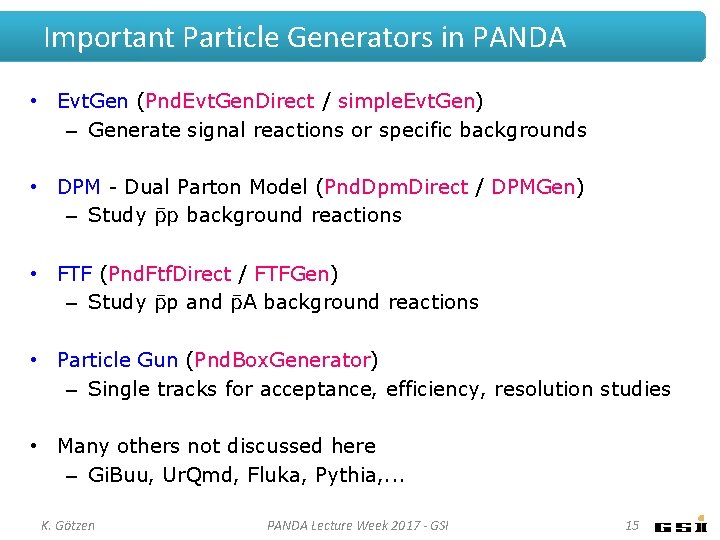
Important Particle Generators in PANDA • Evt. Gen (Pnd. Evt. Gen. Direct / simple. Evt. Gen) – Generate signal reactions or specific backgrounds • DPM - Dual Parton Model (Pnd. Dpm. Direct / DPMGen) – Study p background reactions • FTF (Pnd. Ftf. Direct / FTFGen) – Study p and A background reactions • Particle Gun (Pnd. Box. Generator) – Single tracks for acceptance, efficiency, resolution studies • Many others not discussed here – Gi. Buu, Ur. Qmd, Fluka, Pythia, . . . K. Götzen PANDA Lecture Week 2017 - GSI 15

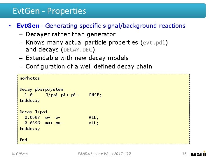
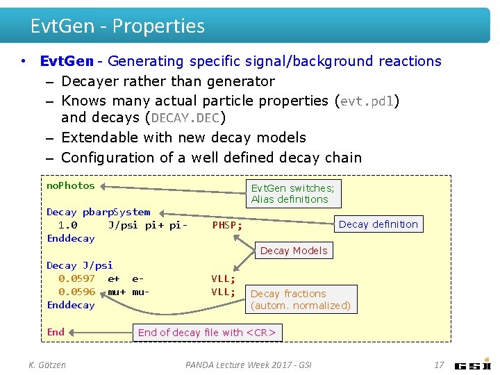
Evt. Gen - Properties • Evt. Gen - Generating specific signal/background reactions – Decayer rather than generator – Knows many actual particle properties (evt. pdl) and decays (DECAY. DEC) – Extendable with new decay models – Configuration of a well defined decay chain no. Photos Decay pbarp. System 1. 0 J/psi pi+ pi. Enddecay PHSP; Decay J/psi 0. 0597 e+ e 0. 0596 mu+ mu. Enddecay VLL; End K. Götzen PANDA Lecture Week 2017 - GSI 16

Evt. Gen - Properties • Evt. Gen - Generating specific signal/background reactions – Decayer rather than generator – Knows many actual particle properties (evt. pdl) and decays (DECAY. DEC) – Extendable with new decay models – Configuration of a well defined decay chain no. Photos Evt. Gen switches; Alias definitions Decay pbarp. System 1. 0 J/psi pi+ pi. Enddecay PHSP; Decay J/psi 0. 0597 e+ e 0. 0596 mu+ mu. Enddecay VLL; End K. Götzen Decay definition Decay Models Decay fractions (autom. normalized) End of decay file with <CR> PANDA Lecture Week 2017 - GSI 17

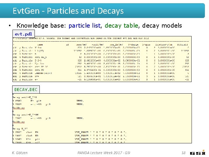
Evt. Gen - Particles and Decays • Knowledge base: particle list, decay table, decay models evt. pdl DECAY. DEC K. Götzen PANDA Lecture Week 2017 - GSI 18

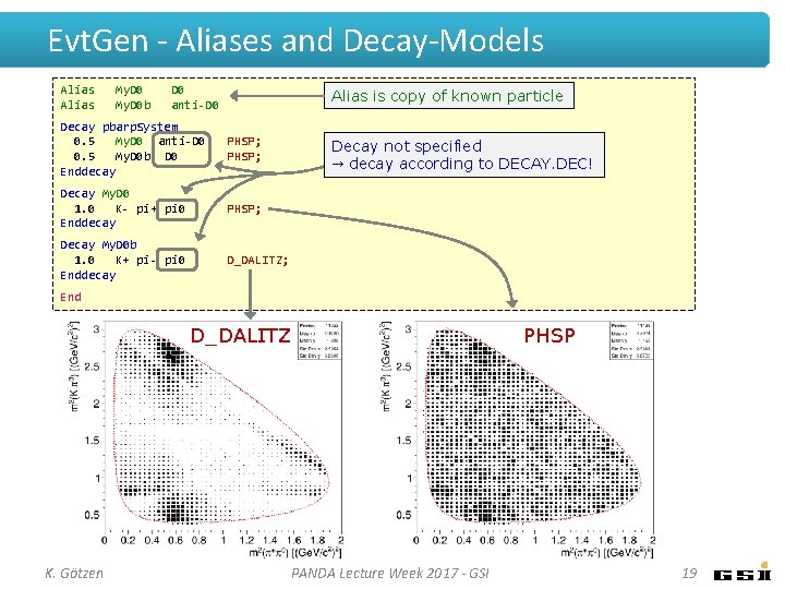
Evt. Gen - Aliases and Decay-Models Alias My. D 0 b D 0 anti-D 0 Alias is copy of known particle Decay pbarp. System 0. 5 My. D 0 anti-D 0 0. 5 My. D 0 b D 0 Enddecay PHSP; Decay My. D 0 1. 0 K- pi+ pi 0 Enddecay PHSP; Decay My. D 0 b 1. 0 K+ pi- pi 0 Enddecay D_DALITZ; Decay not specified → decay according to DECAY. DEC! End D_DALITZ K. Götzen PHSP PANDA Lecture Week 2017 - GSI 19

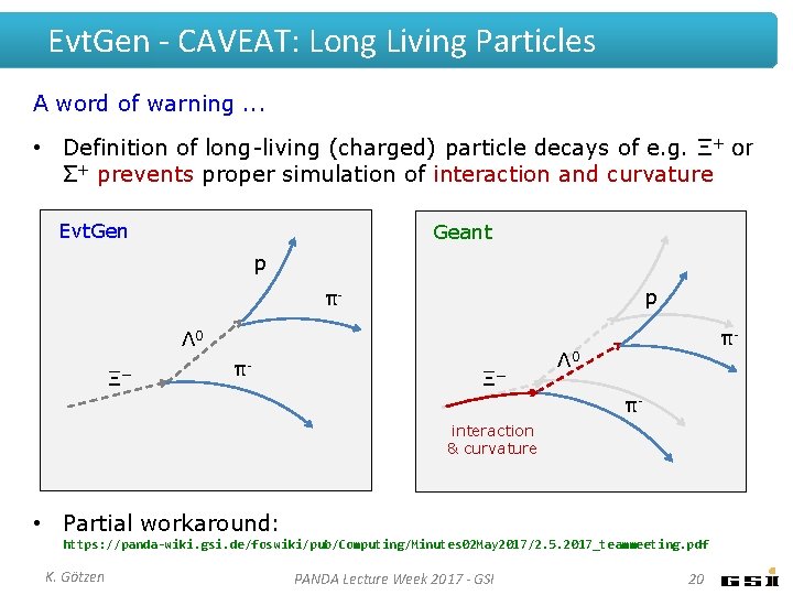
Evt. Gen - CAVEAT: Long Living Particles A word of warning. . . • Definition of long-living (charged) particle decays of e. g. Ξ+ or Σ+ prevents proper simulation of interaction and curvature Evt. Gen Geant p π- p Λ 0 Ξ− π- Λ 0 π- interaction & curvature • Partial workaround: https: //panda-wiki. gsi. de/foswiki/pub/Computing/Minutes 02 May 2017/2. 5. 2017_teammeeting. pdf K. Götzen PANDA Lecture Week 2017 - GSI 20

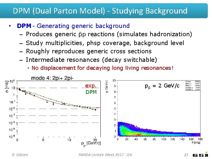
DPM (Dual Parton Model) - Studying Background • DPM - Generating generic background – Produces generic p reactions (simulates hadronization) – Study multiplicities, phsp coverage, background level – Roughly reproduces generic cross sections – Intermediate resonances (decay switchable) • No displacement for decaying long living resonances! exp. DPM K. Götzen PANDA Lecture Week 2017 - GSI p = 2 Ge. V/c 21

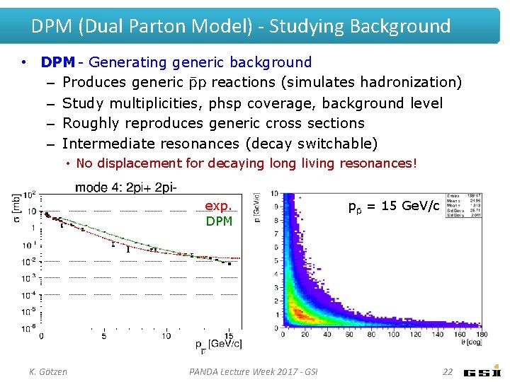
DPM (Dual Parton Model) - Studying Background • DPM - Generating generic background – Produces generic p reactions (simulates hadronization) – Study multiplicities, phsp coverage, background level – Roughly reproduces generic cross sections – Intermediate resonances (decay switchable) • No displacement for decaying long living resonances! exp. DPM K. Götzen PANDA Lecture Week 2017 - GSI p = 15 Ge. V/c 22

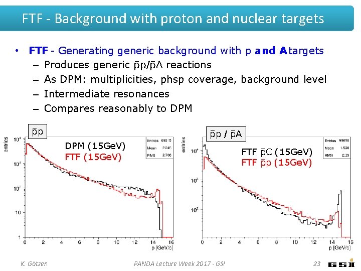
FTF - Background with proton and nuclear targets • FTF - Generating generic background with p and A targets – Produces generic p/ A reactions – As DPM: multiplicities, phsp coverage, background level – Intermediate resonances – Compares reasonably to DPM p p / A DPM (15 Ge. V) FTF (15 Ge. V) K. Götzen FTF C (15 Ge. V) FTF p (15 Ge. V) PANDA Lecture Week 2017 - GSI 23

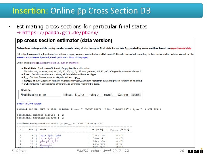
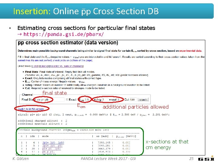
Insertion: Online p Cross Section DB • Estimating cross sections for particular final states → https: //panda. gsi. de/pbarx/ K. Götzen PANDA Lecture Week 2017 - GSI 24

Insertion: Online p Cross Section DB • Estimating cross sections for particular final states → https: //panda. gsi. de/pbarx/ final state Ecm additional particles allowed x-sections at that cm energy K. Götzen PANDA Lecture Week 2017 - GSI 25

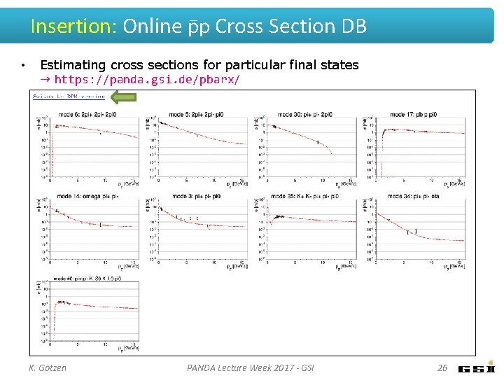
Insertion: Online p Cross Section DB • Estimating cross sections for particular final states → https: //panda. gsi. de/pbarx/ K. Götzen PANDA Lecture Week 2017 - GSI 26

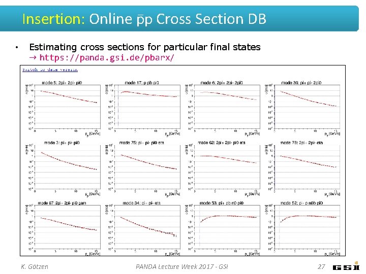
Insertion: Online p Cross Section DB • Estimating cross sections for particular final states → https: //panda. gsi. de/pbarx/ K. Götzen PANDA Lecture Week 2017 - GSI 27

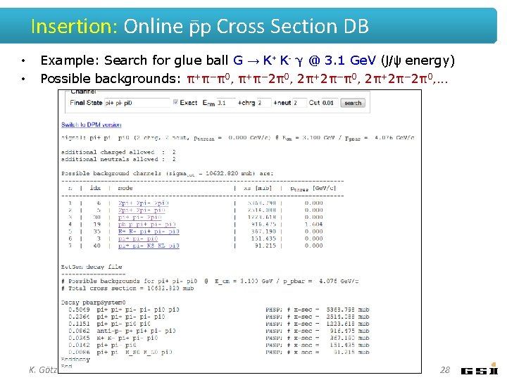
Insertion: Online p Cross Section DB • • Example: Search for glue ball G → K+ K- γ @ 3. 1 Ge. V (J/ψ energy) Possible backgrounds: π+π−π0, π+π− 2π0, 2π+2π− 2π0, . . . K. Götzen PANDA Lecture Week 2017 - GSI 28

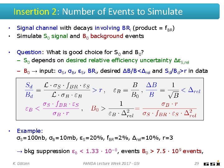
Insertion 2: Number of Events to Simulate • • Signal channel with decays involving BRi (product = f. BR) Simulate S 0 signal and B 0 background events • Question: What is good choice for S 0 and B 0? – S 0 depends on desired relative efficiency uncertainty ΔεS, rel – B 0 → input: σS, σB, εS, BRi, desired ΔB/B<Δrel and Sd/Bd>r in data • Example: σS=100 nb, σB=10 mb, εS=20%, f. BR=2%, Δrel=10%, r=3 → bkg suppression εB < 1. 33 · 10− 8, events B 0 > 7. 5 · 109 events, K. Götzen PANDA Lecture Week 2017 - GSI 29

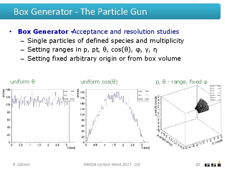
Box Generator - The Particle Gun • Box Generator -Acceptance and resolution studies – Single particles of defined species and multiplicity – Setting ranges in p, pt, θ, cos(θ), φ, y, η – Setting fixed arbitrary origin or from box volume uniform θ K. Götzen uniform cos(θ) PANDA Lecture Week 2017 - GSI p, θ - range, fixed φ 30

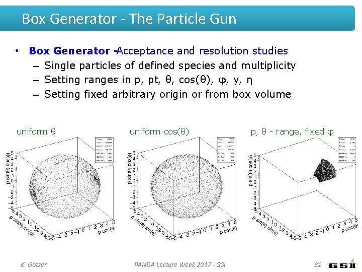
Box Generator - The Particle Gun • Box Generator -Acceptance and resolution studies – Single particles of defined species and multiplicity – Setting ranges in p, pt, θ, cos(θ), φ, y, η – Setting fixed arbitrary origin or from box volume uniform θ K. Götzen uniform cos(θ) PANDA Lecture Week 2017 - GSI p, θ - range, fixed φ 31

GENERATION AND SIMULATION

Generation and Simulation • Three levels of studying particle distrib. with different purpose • Stand-alone usage of generators (Evt. Gen, DPM, FTF) – Study undistorted true distributions – Principle phase space/multiplicity considerations • Fast Simulation – Simplified effective simulation of acceptance & resolution – High speed, easy configurable for physics/detector performance • Full Simulation – Full Geant featured microscopic particle transport – Realistic digis and reconstruction simulation K. Götzen PANDA Lecture Week 2017 - GSI 33

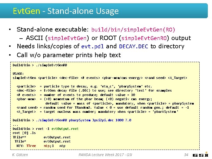
Evt. Gen - Stand-alone Usage • Stand-alone executable: build/bin/simple. Evt. Gen(RO) – ASCII (simple. Evt. Gen) or ROOT (simple. Evt. Gen. RO) output • Needs links/copies of evt. pdl and DECAY. DEC to directory • Call w/o parameter prints help text build/bin >. /simple. Evt. Gen. RO USAGE: simple. Evt. Gen <particle> <dec-file> <# events> <pbar-mom/cms-energy> <rand seed> <A_Target> <particle> <dec-file> <# events> <pbar-mom> = = particle type to decay, e. g. 'eta_c', 'pbarp. System' etc. Evt. Gen decay file (. DEC) to use; see directory 'test' for examples number of events to produce; default value = 10 (>0) momentum of the pbar beam; (<0) negativ cms energy; default value = mass of <particle>, mandatory, when <particle> = pbarp. System <rand seed> = random seed for TRandom 3. Value < 0 = use default random gen. ; default = -1 <A_Target> = target nucleus mass number; mandatory when <particle> = 'pbar. ASystem ' build/bin >. /simple. Evt. Gen. RO pbarp. System Jpsi 2 pi. dec 1000 7. 0. . . build/bin > root -l evt. Output. root [0]. ls TFile** evt. Output. root TFile* evt. Output. root KEY: TTree ntp; 1 ntp K. Götzen PANDA Lecture Week 2017 - GSI 34

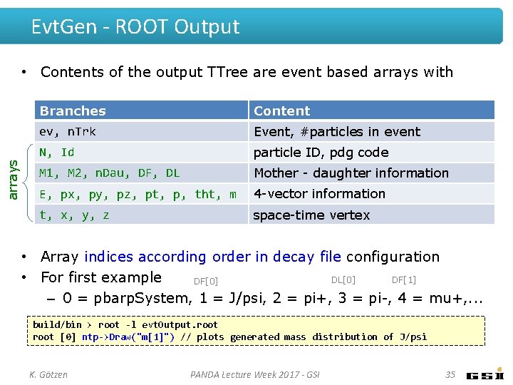
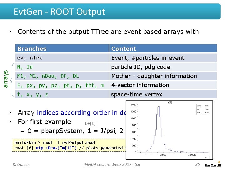
Evt. Gen - ROOT Output arrays • Contents of the output TTree are event based arrays with Branches Content ev, n. Trk Event, #particles in event N, Id particle ID, pdg code M 1, M 2, n. Dau, DF, DL Mother - daughter information E, px, py, pz, pt, p, tht, m 4 -vector information t, x, y, z space-time vertex • Array indices according order in decay file configuration • For first example DL[0] DF[1] DF[0] – 0 = pbarp. System, 1 = J/psi, 2 = pi+, 3 = pi-, 4 = mu+, . . . build/bin > root -l evt. Output. root [0] ntp->Draw("m[1]") // plots generated mass distribution of J/psi K. Götzen PANDA Lecture Week 2017 - GSI 35

Evt. Gen - ROOT Output arrays • Contents of the output TTree are event based arrays with Branches Content ev, n. Trk Event, #particles in event N, Id particle ID, pdg code M 1, M 2, n. Dau, DF, DL Mother - daughter information E, px, py, pz, pt, p, tht, m 4 -vector information t, x, y, z space-time vertex • Array indices according order in decay file configuration • For first example DL[0] DF[1] DF[0] – 0 = pbarp. System, 1 = J/psi, 2 = pi+, 3 = pi-, 4 = mu+, . . . build/bin > root -l evt. Output. root [0] ntp->Draw("m[1]") // plots generated mass distribution of J/psi K. Götzen PANDA Lecture Week 2017 - GSI 36

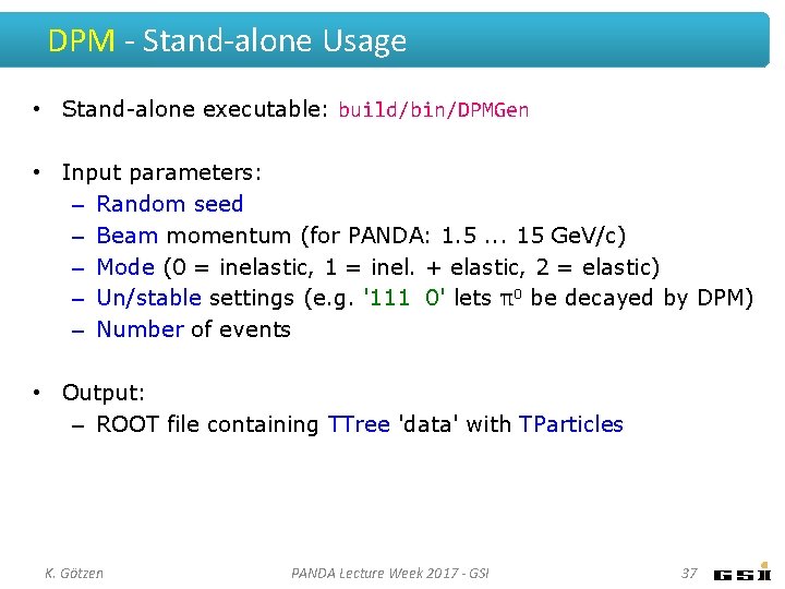
DPM - Stand-alone Usage • Stand-alone executable: build/bin/DPMGen • Input parameters: – Random seed – Beam momentum (for PANDA: 1. 5. . . 15 Ge. V/c) – Mode (0 = inelastic, 1 = inel. + elastic, 2 = elastic) – Un/stable settings (e. g. '111 0' lets π0 be decayed by DPM) – Number of events • Output: – ROOT file containing TTree 'data' with TParticles K. Götzen PANDA Lecture Week 2017 - GSI 37

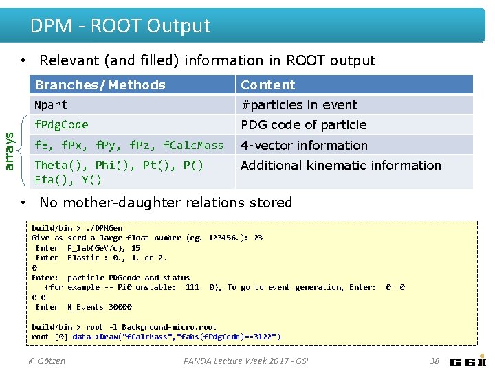
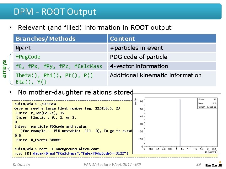
DPM - ROOT Output arrays • Relevant (and filled) information in ROOT output Branches/Methods Content Npart #particles in event f. Pdg. Code PDG code of particle f. E, f. Px, f. Py, f. Pz, f. Calc. Mass 4 -vector information Theta(), Phi(), Pt(), P() Eta(), Y() Additional kinematic information • No mother-daughter relations stored build/bin >. /DPMGen Give as seed a large float number (eg. 123456. ): 23 Enter P_lab(Ge. V/c), 15 Enter Elastic : 0. , 1. or 2. 0 Enter: particle PDGcode and status (for example -- Pi 0 unstable: 111 0), To go to event generation, Enter: 0 0 Enter N_Events 30000 0 0 build/bin > root -l Background-micro. root [0] data->Draw("f. Calc. Mass", "fabs(f. Pdg. Code)==3122") K. Götzen PANDA Lecture Week 2017 - GSI 38

DPM - ROOT Output arrays • Relevant (and filled) information in ROOT output Branches/Methods Content Npart #particles in event f. Pdg. Code PDG code of particle f. E, f. Px, f. Py, f. Pz, f. Calc. Mass 4 -vector information Theta(), Phi(), Pt(), P() Eta(), Y() Additional kinematic information • No mother-daughter relations stored build/bin >. /DPMGen Give as seed a large float number (eg. 123456. ): 23 Enter P_lab(Ge. V/c), 15 Enter Elastic : 0. , 1. or 2. 0 Enter: particle PDGcode and status (for example -- Pi 0 unstable: 111 0), To go to event generation, Enter: 0 0 Enter N_Events 30000 0 0 build/bin > root -l Background-micro. root [0] data->Draw("f. Calc. Mass", "fabs(f. Pdg. Code)==3122") K. Götzen PANDA Lecture Week 2017 - GSI 39

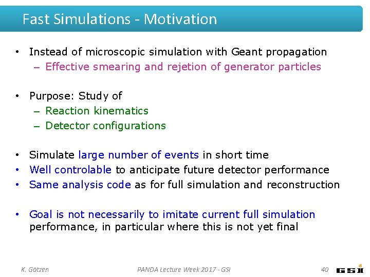
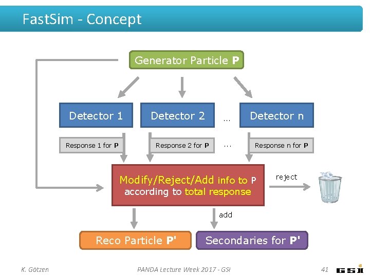
Fast Simulations - Motivation • Instead of microscopic simulation with Geant propagation – Effective smearing and rejetion of generator particles • Purpose: Study of – Reaction kinematics – Detector configurations • Simulate large number of events in short time • Well controlable to anticipate future detector performance • Same analysis code as for full simulation and reconstruction • Goal is not necessarily to imitate current full simulation performance, in particular where this is not yet final K. Götzen PANDA Lecture Week 2017 - GSI 40

Fast. Sim - Concept Generator Particle P Detector 1 Response 1 for P Detector 2 . . . Response 2 for P Detector n . . . Response n for P Modify/Reject/Add info to P reject according to total response add Reco Particle P' K. Götzen Secondaries for P' PANDA Lecture Week 2017 - GSI 41

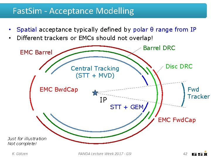
Fast. Sim - Acceptance Modelling • Spatial acceptance typically defined by polar θ range from IP • Different trackers or EMCs should not overlap! Barrel DRC EMC Barrel Central Tracking (STT + MVD) Disc DRC EMC Bwd. Cap IP Fwd Tracker STT + GEM EMC Fwd. Cap Just for illustration Not complete! K. Götzen PANDA Lecture Week 2017 - GSI 42

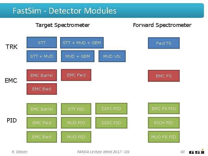
Fast. Sim - Detector Modules Target Spectrometer TRK STT + MVD EMC Barrel Forward Spectrometer STT + MVD + GEM Fwd TS MVD Vtx EMC Fwd EMC FS EMC Bwd PID K. Götzen EMC Barrel STT PID DIRC PID EMC FS PID EMC Fwd MVD PID DISC PID RICH PID EMC Bwd MUO PID PANDA Lecture Week 2017 - GSI MUO FS PID 43

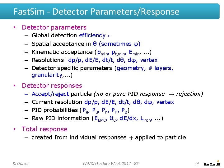
Fast. Sim - Detector Parameters/Response • Detector parameters – – – Global detection efficiency ε Spatial acceptance in θ (sometimes φ) Kinematic acceptance (pmin, pt, min, Emin, . . . ) Resolutions: dp/p, d. E/E, dt/t, dθ, dφ, vertex Detector specific parameters (geometry, # layers, granularity, . . . ) • Detector responses – – Accept/reject particle (no or pure PID response → rejection) Current resolution dp/p, d. E/E, dt/t, dθ, dφ, vertex PID probabilities (Pe, Pμ, Pπ, PK, Pp) Raw PID information (EEMC, θC, d. E/dx, Liron, . . . ) • Total response – created from individual responses + applied to particle K. Götzen PANDA Lecture Week 2017 - GSI 44

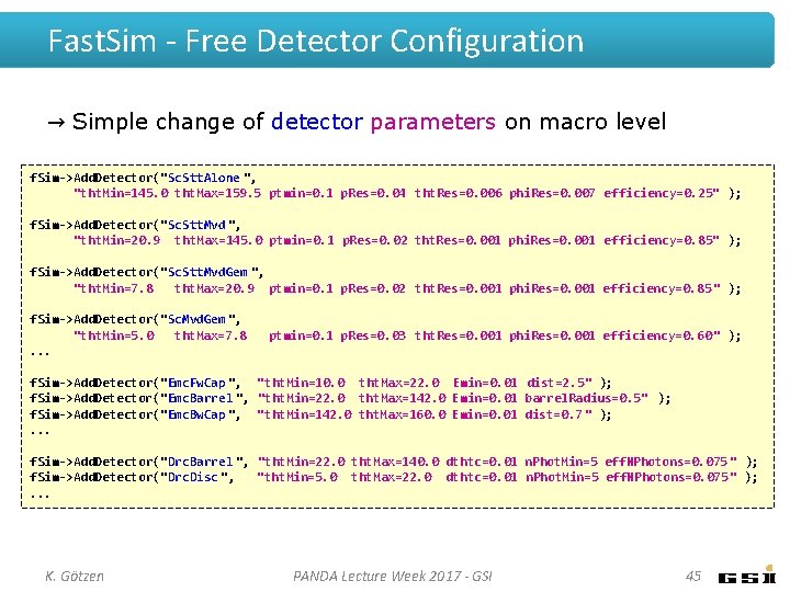
Fast. Sim - Free Detector Configuration → Simple change of detector parameters on macro level f. Sim->Add. Detector("Sc. Stt. Alone ", "tht. Min=145. 0 tht. Max=159. 5 ptmin=0. 1 p. Res=0. 04 tht. Res=0. 006 phi. Res=0. 007 efficiency=0. 25" ); f. Sim->Add. Detector("Sc. Stt. Mvd ", "tht. Min=20. 9 tht. Max=145. 0 ptmin=0. 1 p. Res=0. 02 tht. Res=0. 001 phi. Res=0. 001 efficiency=0. 85" ); f. Sim->Add. Detector("Sc. Stt. Mvd. Gem ", "tht. Min=7. 8 tht. Max=20. 9 ptmin=0. 1 p. Res=0. 02 tht. Res=0. 001 phi. Res=0. 001 efficiency=0. 85 " ); f. Sim->Add. Detector("Sc. Mvd. Gem ", "tht. Min=5. 0 tht. Max=7. 8. . . ptmin=0. 1 p. Res=0. 03 tht. Res=0. 001 phi. Res=0. 001 efficiency=0. 60 " ); f. Sim->Add. Detector("Emc. Fw. Cap ", "tht. Min=10. 0 tht. Max=22. 0 Emin=0. 01 dist=2. 5" ); f. Sim->Add. Detector("Emc. Barrel ", "tht. Min=22. 0 tht. Max=142. 0 Emin=0. 01 barrel. Radius=0. 5" ); f. Sim->Add. Detector("Emc. Bw. Cap ", "tht. Min=142. 0 tht. Max=160. 0 Emin=0. 01 dist=0. 7 " ); . . . f. Sim->Add. Detector("Drc. Barrel ", "tht. Min=22. 0 tht. Max=140. 0 dthtc=0. 01 n. Phot. Min=5 eff. NPhotons=0. 075 " ); f. Sim->Add. Detector("Drc. Disc ", "tht. Min=5. 0 tht. Max=22. 0 dthtc=0. 01 n. Phot. Min=5 eff. NPhotons=0. 075" ); . . . K. Götzen PANDA Lecture Week 2017 - GSI 45

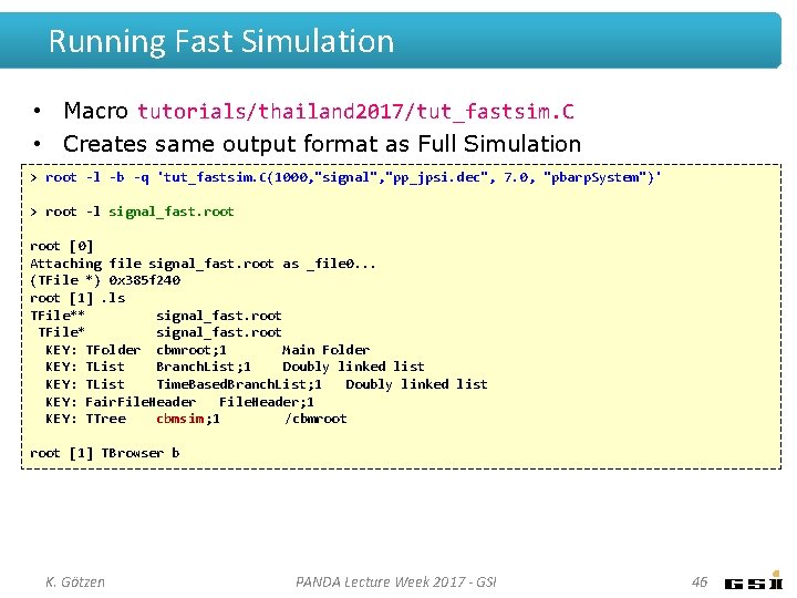
Running Fast Simulation • Macro tutorials/thailand 2017/tut_fastsim. C • Creates same output format as Full Simulation > root -l -b -q 'tut_fastsim. C(1000, "signal", "pp_jpsi. dec", 7. 0, "pbarp. System")' > root -l signal_fast. root [0] Attaching file signal_fast. root as _file 0. . . (TFile *) 0 x 385 f 240 root [1]. ls TFile** signal_fast. root TFile* signal_fast. root KEY: TFolder cbmroot; 1 Main Folder KEY: TList Branch. List; 1 Doubly linked list KEY: TList Time. Based. Branch. List; 1 Doubly linked list KEY: Fair. File. Header; 1 KEY: TTree cbmsim ; 1 /cbmroot [1] TBrowser b K. Götzen PANDA Lecture Week 2017 - GSI 46

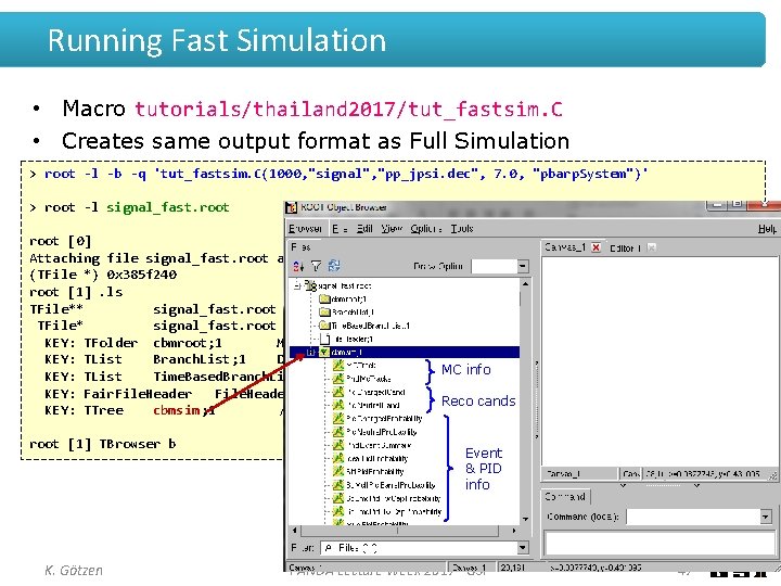
Running Fast Simulation • Macro tutorials/thailand 2017/tut_fastsim. C • Creates same output format as Full Simulation > root -l -b -q 'tut_fastsim. C(1000, "signal", "pp_jpsi. dec", 7. 0, "pbarp. System")' > root -l signal_fast. root [0] Attaching file signal_fast. root as _file 0. . . (TFile *) 0 x 385 f 240 root [1]. ls TFile** signal_fast. root TFile* signal_fast. root KEY: TFolder cbmroot; 1 Main Folder KEY: TList Branch. List; 1 Doubly linked list info KEY: TList Time. Based. Branch. List; 1 Doubly linked MC list KEY: Fair. File. Header; 1 Reco cands KEY: TTree cbmsim ; 1 /cbmroot [1] TBrowser b K. Götzen Event & PID info PANDA Lecture Week 2017 - GSI 47

EXERCISES

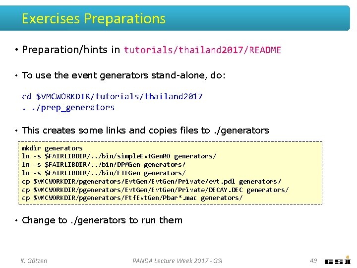
Exercises Preparations • Preparation/hints in tutorials/thailand 2017/README • To use the event generators stand-alone, do: cd $VMCWORKDIR/tutorials/thailand 2017. . /prep_generators • This creates some links and copies files to. /generators mkdir generators ln -s $FAIRLIBDIR/. . /bin/simple. Evt. Gen. RO generators/ ln -s $FAIRLIBDIR/. . /bin/DPMGen generators/ ln -s $FAIRLIBDIR/. . /bin/FTFGen generators/ cp $VMCWORKDIR/pgenerators/Evt. Gen/Private/evt. pdl generators/ cp $VMCWORKDIR/pgenerators/Evt. Gen/Private/DECAY. DEC generators/ cp $VMCWORKDIR/pgenerators/Ftf. Evt. Gen/Pbar*. mac generators/ • Change to. /generators to run them K. Götzen PANDA Lecture Week 2017 - GSI 49

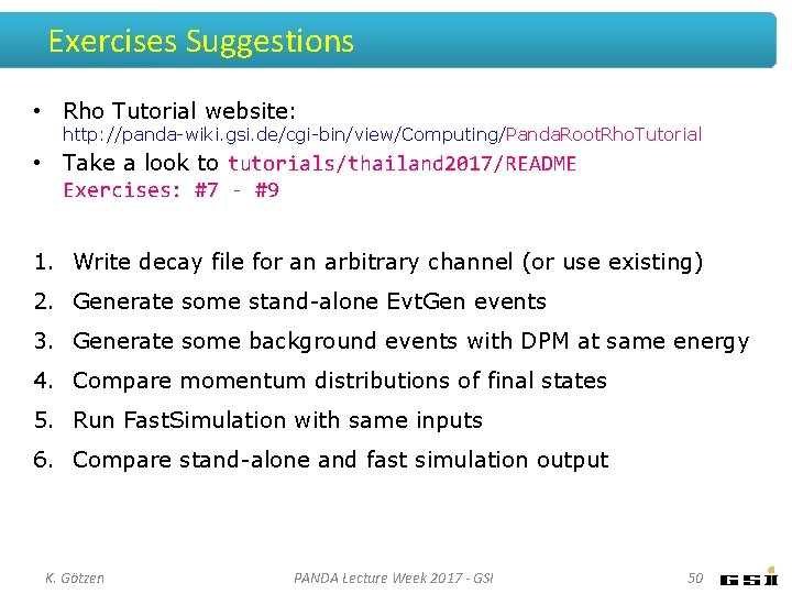
Exercises Suggestions • Rho Tutorial website: http: //panda-wiki. gsi. de/cgi-bin/view/Computing/Panda. Root. Rho. Tutorial • Take a look to tutorials/thailand 2017/README Exercises: #7 - #9 1. Write decay file for an arbitrary channel (or use existing) 2. Generate some stand-alone Evt. Gen events 3. Generate some background events with DPM at same energy 4. Compare momentum distributions of final states 5. Run Fast. Simulation with same inputs 6. Compare stand-alone and fast simulation output K. Götzen PANDA Lecture Week 2017 - GSI 50

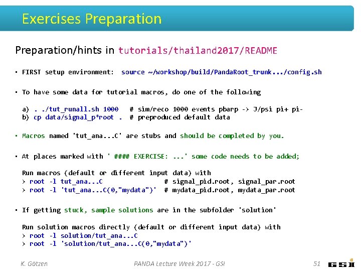
Exercises Preparation/hints in tutorials/thailand 2017/README • FIRST setup environment: source ~/workshop/build/Panda. Root_trunk. . . /config. sh • To have some data for tutorial macros, do one of the following a). . /tut_runall. sh 1000 b) cp data/signal_p*root. # sim/reco 1000 events pbarp -> J/psi pi+ pi# preproduced default data • Macros named 'tut_ana. . . C' are stubs and should be completed by you. • At places marked with ' #### EXERCISE: . . . ' some code needs to be added; Run macros (default or different input data) with > root -l tut_ana. . . C # signal_pid. root, signal_par. root > root -l 'tut_ana. . . C(0, "mydata")' # mydata_pid. root, mydata_par. root • If getting stuck, sample solutions are in the subfolder 'solution' Run solution macros directly (default or different input data) with > root -l solution/tut_ana. . . C > root -l 'solution/tut_ana. . . C(0, "mydata")' K. Götzen PANDA Lecture Week 2017 - GSI 51