Physics Analysis Concepts with Panda Root 2 PANDA

Physics Analysis Concepts with Panda. Root (2) PANDA Lecture Week 2017 GSI, Dec 11 - 15, 2017 Klaus Götzen GSI Darmstadt

Topics • Particle Identification • Particle Selectors (Pnd. Pid. Combiner, Pnd. Pid. Selector) • MC Truth Match (Pnd. Analysis: : Mc. Truth. Match) • Fitting Basics • Fitting Tools (Pnd. Kin. Vtx. Fitter, Pnd. Kin. Fitter) • Uncertainties K. Götzen PANDA Lecture Week 2017 - GSI 2

PARTICLE IDENTIFICATION

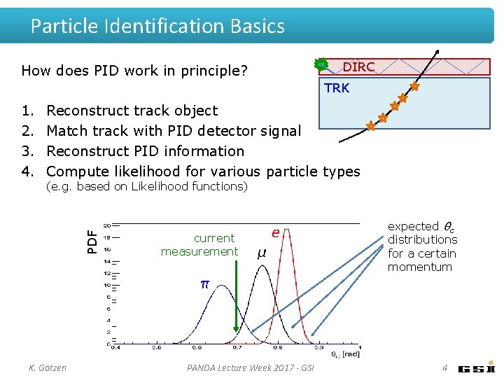
Particle Identification Basics How does PID work in principle? DIRC TRK Reconstruct track object Match track with PID detector signal Reconstruct PID information Compute likelihood for various particle types (e. g. based on Likelihood functions) PDF 1. 2. 3. 4. K. Götzen current measurement PANDA Lecture Week 2017 - GSI expected θc distributions for a certain momentum 4

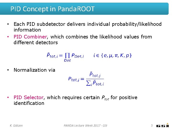
PID Concept in Panda. ROOT • Each PID subdetector delivers individual probability/likelihood information • PID Combiner, which combines the likelihood values from different detectors • Normalization via • PID Selector, which requires certain Ptot for positive identification K. Götzen PANDA Lecture Week 2017 - GSI 5

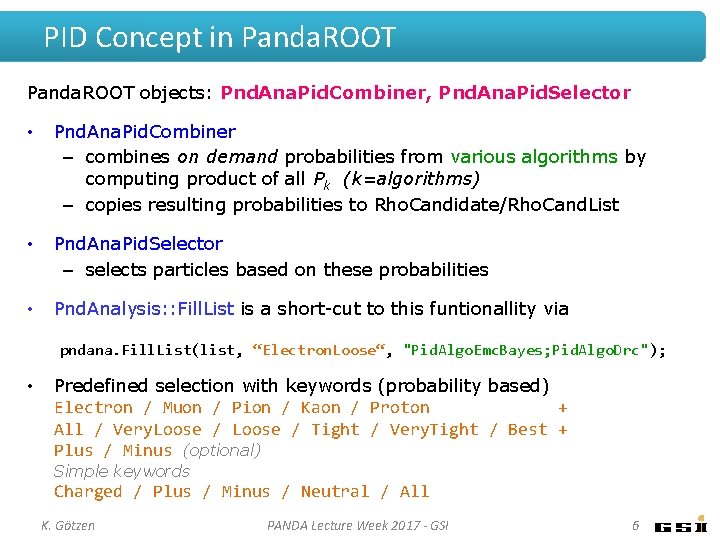
PID Concept in Panda. ROOT objects: Pnd. Ana. Pid. Combiner, Pnd. Ana. Pid. Selector • Pnd. Ana. Pid. Combiner – combines on demand probabilities from various algorithms by computing product of all Pk (k=algorithms) – copies resulting probabilities to Rho. Candidate/Rho. Cand. List • Pnd. Ana. Pid. Selector – selects particles based on these probabilities • Pnd. Analysis: : Fill. List is a short-cut to this funtionallity via pndana. Fill. List(list, “Electron. Loose“, "Pid. Algo. Emc. Bayes; Pid. Algo. Drc"); • Predefined selection with keywords (probability based) Electron / Muon / Pion / Kaon / Proton + All / Very. Loose / Tight / Very. Tight / Best + Plus / Minus (optional) Simple keywords Charged / Plus / Minus / Neutral / All K. Götzen PANDA Lecture Week 2017 - GSI 6

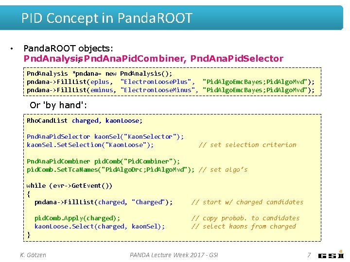
PID Concept in Panda. ROOT • Panda. ROOT objects: Pnd. Analysis , Pnd. Ana. Pid. Combiner, Pnd. Ana. Pid. Selector Pnd. Analysis *pndana= new Pnd. Analysis(); pndana->Fill. List(eplus, "Electron. Loose. Plus", "Pid. Algo. Emc. Bayes; Pid. Algo. Mvd"); pndana->Fill. List(eminus, "Electron. Loose. Minus", "Pid. Algo. Emc. Bayes; Pid. Algo. Mvd"); Or 'by hand': Rho. Cand. List charged, kaon. Loose; Pnd. Ana. Pid. Selector kaon. Sel("Kaon. Selector"); kaon. Sel. Set. Selection("Kaon. Loose"); // set selection criterion Pnd. Ana. Pid. Combiner pid. Comb("Pid. Combiner"); pid. Comb. Set. Tca. Names("Pid. Algo. Drc; Pid. Algo. Mvd"); // set algo‘s while (evr->Get. Event()) { pndana->Fill. List(charged, "Charged"); // start w/ charged candidates pid. Comb. Apply(charged); kaon. Loose. Select(charged, kaon. Sel); // copy probab. to candidates // select kaons from charged } K. Götzen PANDA Lecture Week 2017 - GSI 7

MONTE CARLO TRUTH

Monte Carlo Truth Match • In simulated reactions → possibility to map reco object to MC object Tracking detector MC track 1 MC track 2 K. Götzen PANDA Lecture Week 2017 - GSI 9

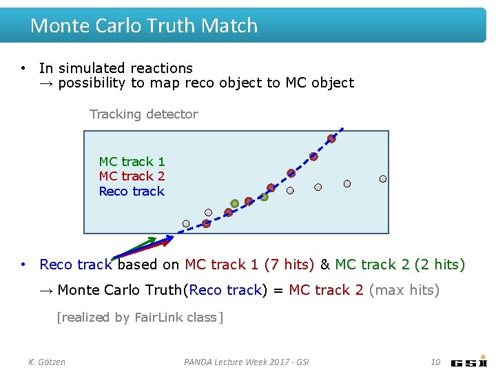
Monte Carlo Truth Match • In simulated reactions → possibility to map reco object to MC object Tracking detector MC track 1 MC track 2 Reco track • Reco track based on MC track 1 (7 hits) & MC track 2 (2 hits) → Monte Carlo Truth(Reco track) = MC track 2 (max hits) [realized by Fair. Link class] K. Götzen PANDA Lecture Week 2017 - GSI 10

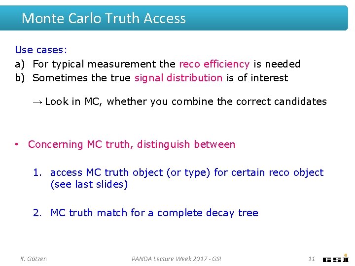
Monte Carlo Truth Access Use cases: a) For typical measurement the reco efficiency is needed b) Sometimes the true signal distribution is of interest → Look in MC, whether you combine the correct candidates • Concerning MC truth, distinguish between 1. access MC truth object (or type) for certain reco object (see last slides) 2. MC truth match for a complete decay tree K. Götzen PANDA Lecture Week 2017 - GSI 11

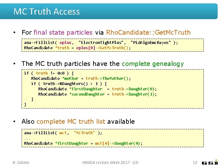
MC Truth Access • For final state particles via Rho. Candidate: : Get. Mc. Truth ana->Fill. List( eplus, "Electron. Tight. Plus", "Pid. Algo. Emc. Bayes" ); Rho. Candidate *truth = eplus[0]->Get. Mc. Truth(); • The MC truth particles have the complete genealogy if ( truth != 0 x 0 ) { Rho. Candidate *mother = truth->The. Mother(); if ( truth->NDaughters() > 1 ) { Rho. Candidate *first. Daughter = truth->Daughter(0); Rho. Candidate *second. Daughter = truth->Daughter(1); } } • Also complete MC truth list available ana->Fill. List( mct, "Mc. Truth" ); . . . Rho. Candidate *first. Daughter = mct[0]->Daughter(0); K. Götzen PANDA Lecture Week 2017 - GSI 12

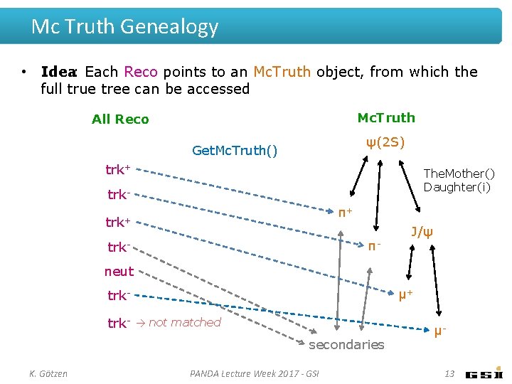
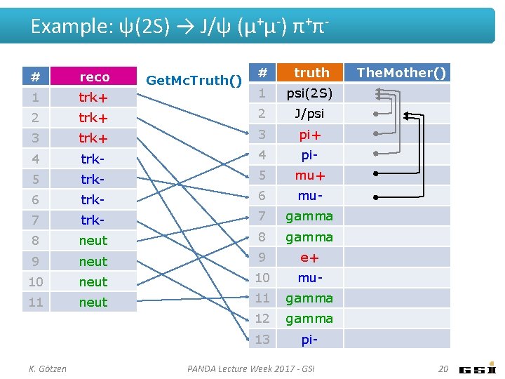
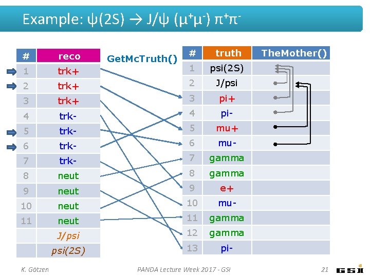
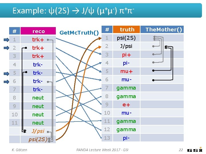
Mc Truth Genealogy • Idea: Each Reco points to an Mc. Truth object, from which the full true tree can be accessed Mc. Truth All Reco ψ(2 S) Get. Mc. Truth() trk+ The. Mother() Daughter(i) trkπ+ trk+ π- trk- J/ψ neut μ+ trktrk- → not matched secondaries K. Götzen PANDA Lecture Week 2017 - GSI μ 13

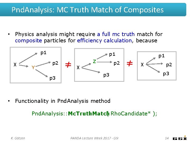
Pnd. Analysis: MC Truth Match of Composites • Physics analysis might require a full mc truth match for composite particles for efficiency calculation, because p 1 X Y p 1 p 2 p 3 ≠ Z p 2 X ≠ p 1 X p 3 p 2 p 3 • Functionality in Pnd. Analysis method Pnd. Analysis: : Mc. Truth. Match ( Rho. Candidate* ); K. Götzen PANDA Lecture Week 2017 - GSI 14

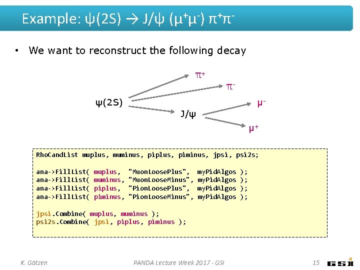
Example: ψ(2 S) → J/ψ (μ+μ-) π+π • We want to reconstruct the following decay π+ π- ψ(2 S) μJ/ψ μ+ Rho. Cand. List muplus, muminus, piplus, piminus, jpsi, psi 2 s; ana->Fill. List( muplus, muminus, piplus, piminus, "Muon. Loose. Plus", "Muon. Loose. Minus", "Pion. Loose. Plus", "Pion. Loose. Minus", my. Pid. Algos ); ); jpsi. Combine( muplus, muminus ); psi 2 s. Combine( jpsi, piplus, piminus ); K. Götzen PANDA Lecture Week 2017 - GSI 15

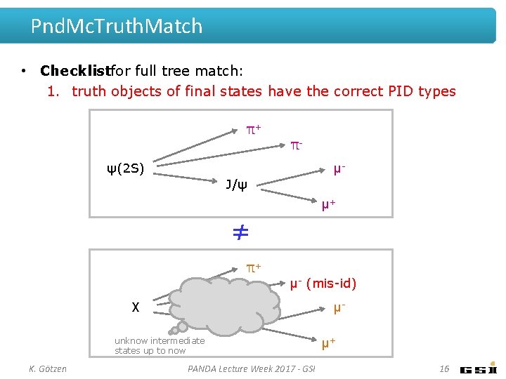
Pnd. Mc. Truth. Match • Checklistfor full tree match: 1. truth objects of final states have the correct PID types π+ π- ψ(2 S) μJ/ψ μ+ ≠ π+ μ- (mis-id) X μY unknow intermediate states up to now K. Götzen PANDA Lecture Week 2017 - GSI μ+ 16

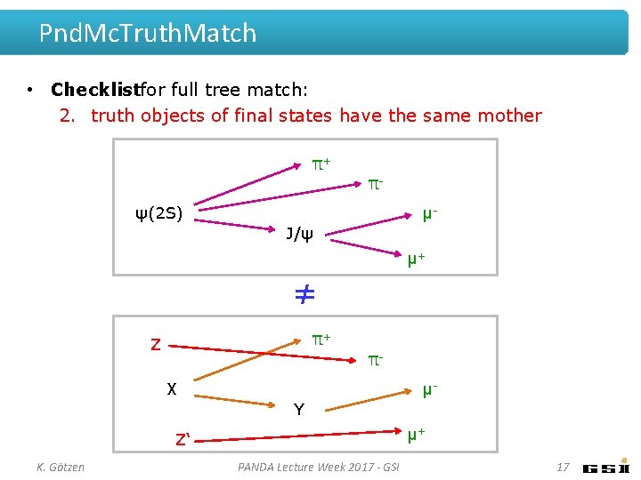
Pnd. Mc. Truth. Match • Checklistfor full tree match: 2. truth objects of final states have the same mother π+ π- ψ(2 S) μJ/ψ μ+ ≠ π+ Z π- X μY μ+ Z‘ K. Götzen PANDA Lecture Week 2017 - GSI 17

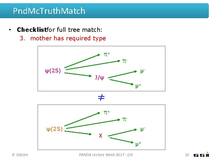
Pnd. Mc. Truth. Match • Checklistfor full tree match: 3. mother has required type π+ π- ψ(2 S) μJ/ψ μ+ ≠ π+ π- ψ(2 S) μX μ+ K. Götzen PANDA Lecture Week 2017 - GSI 18

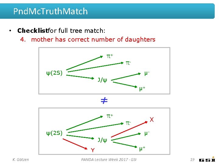
Pnd. Mc. Truth. Match • Checklistfor full tree match: 4. mother has correct number of daughters π+ π- ψ(2 S) μJ/ψ μ+ ≠ π+ X π- ψ(2 S) μJ/ψ Y K. Götzen PANDA Lecture Week 2017 - GSI μ+ 19

Example: ψ(2 S) → J/ψ (μ+μ-) π+π# truth trk+ 1 psi(2 S) 2 trk+ 2 J/psi 3 trk+ 3 pi+ 4 trk- 4 pi- 5 trk- 5 mu+ 6 trk- 6 mu- 7 trk- 7 gamma 8 neut 8 gamma 9 neut 9 e+ 10 neut 10 mu- 11 neut 11 gamma 12 gamma 13 pi- # reco 1 K. Götzen Get. Mc. Truth() PANDA Lecture Week 2017 - GSI The. Mother() 20

Example: ψ(2 S) → J/ψ (μ+μ-) π+π# truth trk+ 1 psi(2 S) 2 trk+ 2 J/psi 3 trk+ 3 pi+ 4 trk- 4 pi- 5 trk- 5 mu+ 6 trk- 6 mu- 7 trk- 7 gamma 8 neut 8 gamma 9 neut 9 e+ 10 neut 10 mu- 11 neut 11 gamma J/psi 12 gamma psi(2 S) 13 pi- # reco 1 K. Götzen Get. Mc. Truth() PANDA Lecture Week 2017 - GSI The. Mother() 21

Example: ψ(2 S) → J/ψ (μ+μ-) π+π# truth trk+ 1 psi(2 S) 2 trk+ 2 J/psi 3 trk+ 3 pi+ 4 trk- 4 pi- 5 trk- 5 mu+ 6 trk- 6 mu- 7 trk- 7 gamma 8 neut 8 gamma 9 neut 9 e+ 10 neut 10 mu- 11 neut 11 gamma J/psi 12 gamma psi(2 S) 13 pi- # reco 1 K. Götzen Get. Mc. Truth() PANDA Lecture Week 2017 - GSI The. Mother() 22

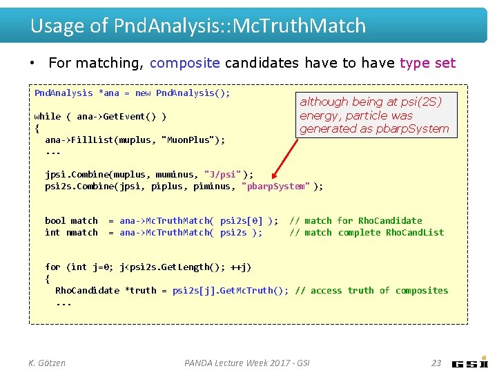
Usage of Pnd. Analysis: : Mc. Truth. Match • For matching, composite candidates have to have type set Pnd. Analysis *ana = new Pnd. Analysis(); while ( ana->Get. Event() ) { ana->Fill. List(muplus, "Muon. Plus"); . . . although being at psi(2 S) energy, particle was generated as pbarp. System jpsi. Combine(muplus, muminus, "J/psi" ); psi 2 s. Combine(jpsi, piplus, piminus, "pbarp. System" ); bool match int nmatch = ana->Mc. Truth. Match( psi 2 s[0] ); = ana->Mc. Truth. Match( psi 2 s ); // match for Rho. Candidate // match complete Rho. Cand. List for (int j=0; j<psi 2 s. Get. Length(); ++j) { Rho. Candidate *truth = psi 2 s[j]. Get. Mc. Truth(); // access truth of composites. . . K. Götzen PANDA Lecture Week 2017 - GSI 23

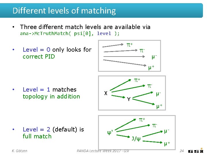
Different levels of matching • Three different match levels are available via ana->Mc. Truth. Match( psi[0], level ); • π+ Level = 0 only looks for correct PID π- μμ+ π+ • Level = 1 matches topology in addition X πμ- Y μ+ π+ • Level = 2 (default) is full match K. Götzen ψ‘ PANDA Lecture Week 2017 - GSI J/ψ π- μμ+ 24

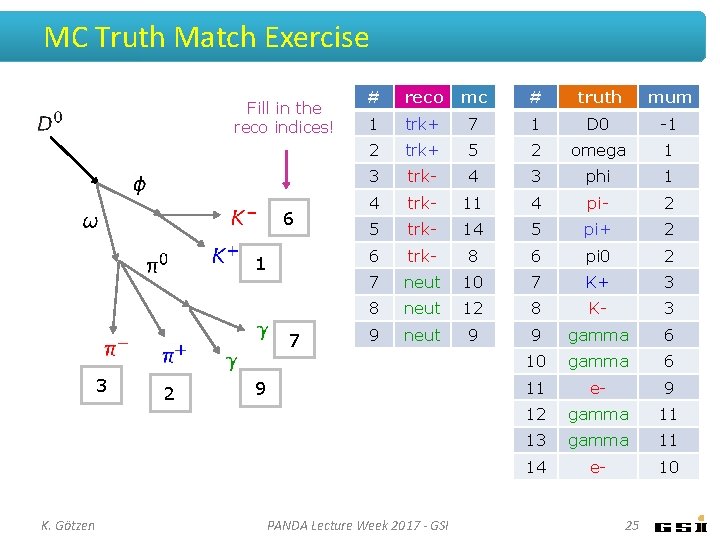
MC Truth Match Exercise Fill in the reco indices! 6 1 7 3 K. Götzen 2 # reco mc # truth mum 1 trk+ 7 1 D 0 -1 2 trk+ 5 2 omega 1 3 trk- 4 3 phi 1 4 trk- 11 4 pi- 2 5 trk- 14 5 pi+ 2 6 trk- 8 6 pi 0 2 7 neut 10 7 K+ 3 8 neut 12 8 K- 3 9 neut 9 9 gamma 6 10 gamma 6 11 e- 9 12 gamma 11 13 gamma 11 14 e- 10 9 PANDA Lecture Week 2017 - GSI 25

FITTING

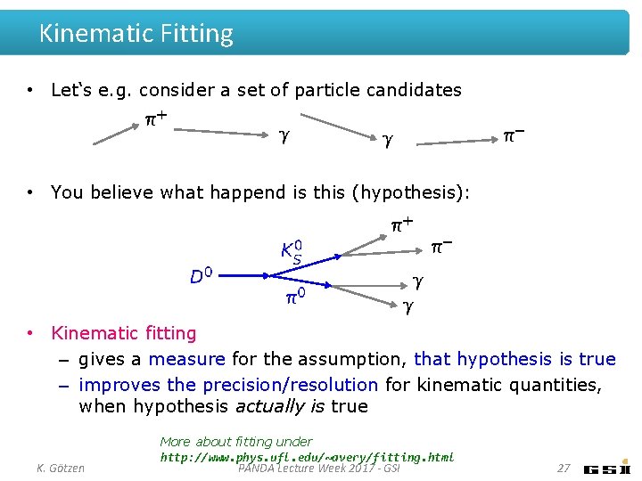
Kinematic Fitting • Let‘s e. g. consider a set of particle candidates • You believe what happend is this (hypothesis): • Kinematic fitting – gives a measure for the assumption, that hypothesis is true – improves the precision/resolution for kinematic quantities, when hypothesis actually is true K. Götzen More about fitting under http: //www. phys. ufl. edu/~avery/fitting. html PANDA Lecture Week 2017 - GSI 27

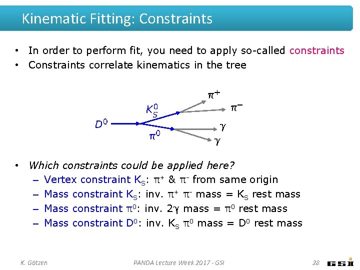
Kinematic Fitting: Constraints • In order to perform fit, you need to apply so-called constraints • Constraints correlate kinematics in the tree • Which constraints could be applied here? – Vertex constraint KS: π+ & π- from same origin – Mass constraint KS: inv. π+ π- mass = KS rest mass – Mass constraint π0: inv. 2γ mass = π0 rest mass – Mass constraint D 0: inv. KS π0 mass = D 0 rest mass K. Götzen PANDA Lecture Week 2017 - GSI 28

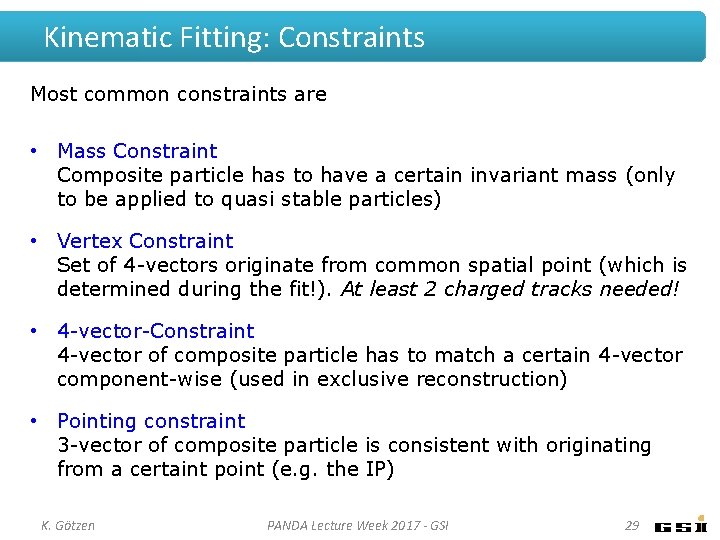
Kinematic Fitting: Constraints Most common constraints are • Mass Constraint Composite particle has to have a certain invariant mass (only to be applied to quasi stable particles) • Vertex Constraint Set of 4 -vectors originate from common spatial point (which is determined during the fit!). At least 2 charged tracks needed! • 4 -vector-Constraint 4 -vector of composite particle has to match a certain 4 -vector component-wise (used in exclusive reconstruction) • Pointing constraint 3 -vector of composite particle is consistent with originating from a certaint point (e. g. the IP) K. Götzen PANDA Lecture Week 2017 - GSI 29

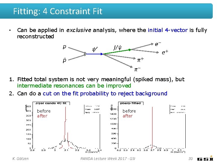
Fitting: 4 Constraint Fit • Can be applied in exclusive analysis, where the initial 4 -vector is fully reconstructed 1. Fitted total system is not very meaningful (spiked mass), but intermediate resonances can be improved 2. Can do a cut on the fit probability to reject background before after K. Götzen before after PANDA Lecture Week 2017 - GSI 30

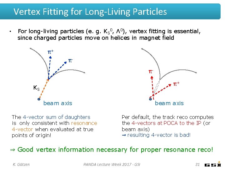
Vertex Fitting for Long-Living Particles • For long-living particles (e. g. KS 0, Λ 0), vertex fitting is essential, since charged particles move on helices in magnet field π+ πππ+ KS beam axis The 4 -vector sum of daughters is only consistent with resonance 4 -vector when evaluated at true points of origin! Per default, the track reco computes the 4 -vectors at POCA to the IP (or beam axis) → resulting 4 -vector is bad! ⇒ Good vertex information necessary for proper resonance reco! K. Götzen PANDA Lecture Week 2017 - GSI 31

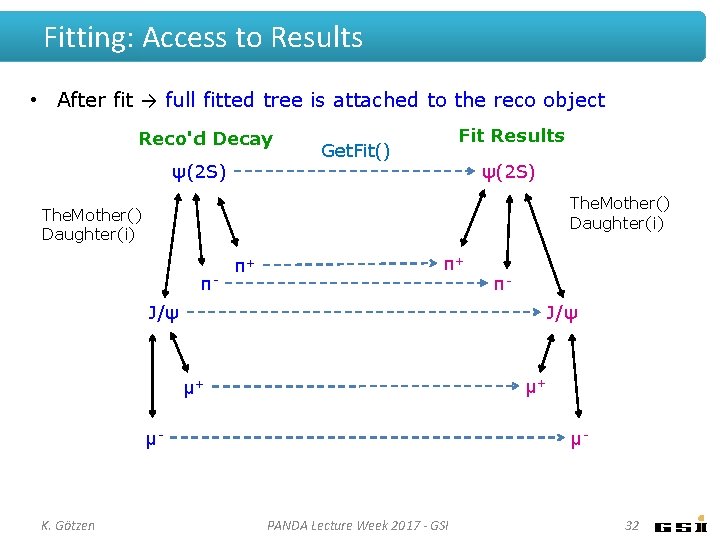
Fitting: Access to Results • After fit → full fitted tree is attached to the reco object Reco'd Decay ψ(2 S) Fit Results Get. Fit() ψ(2 S) The. Mother() Daughter(i) π- π+ π+ π- J/ψ μ+ μ+ μ- K. Götzen μ- PANDA Lecture Week 2017 - GSI 32

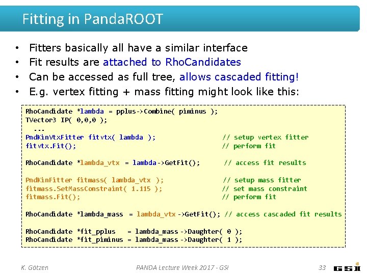
Fitting in Panda. ROOT • • Fitters basically all have a similar interface Fit results are attached to Rho. Candidates Can be accessed as full tree, allows cascaded fitting! E. g. vertex fitting + mass fitting might look like this: Rho. Candidate *lambda = pplus->Combine( piminus ); TVector 3 IP( 0, 0, 0 ); . . . Pnd. Kin. Vtx. Fitter fitvtx( lambda ); // setup vertex fitter fitvtx. Fit(); // perform fit Rho. Candidate *lambda_vtx = lambda ->Get. Fit(); Pnd. Kin. Fitter fitmass( lambda_vtx ); fitmass. Set. Mass. Constraint( 1. 115 ); fitmass. Fit(); // access fit results // setup mass fitter // set mass constraint // perform fit Rho. Candidate *lambda_mass = lambda_vtx ->Get. Fit(); // access cascaded fit results Rho. Candidate *fit_pplus = lambda_mass ->Daughter( 0 ); Rho. Candidate *fit_piminus = lambda_mass ->Daughter( 1 ); K. Götzen PANDA Lecture Week 2017 - GSI 33

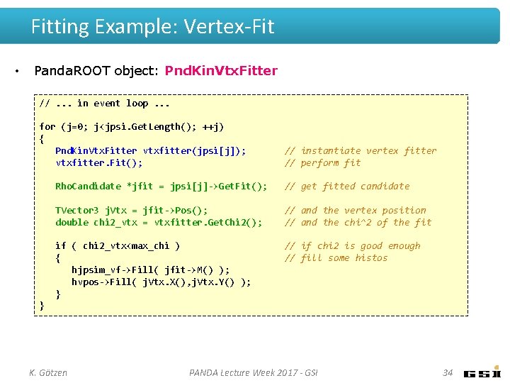
Fitting Example: Vertex-Fit • Panda. ROOT object: Pnd. Kin. Vtx. Fitter //. . . in event loop. . . for (j=0; j<jpsi. Get. Length(); ++j) { Pnd. Kin. Vtx. Fitter vtxfitter(jpsi[j]); vtxfitter. Fit(); // instantiate vertex fitter // perform fit Rho. Candidate *jfit = jpsi[j]->Get. Fit(); // get fitted candidate TVector 3 j. Vtx = jfit->Pos(); double chi 2_vtx = vtxfitter. Get. Chi 2(); // and the vertex position // and the chi^2 of the fit if ( chi 2_vtx<max_chi ) { hjpsim_vf->Fill( jfit->M() ); hvpos->Fill( j. Vtx. X(), j. Vtx. Y() ); } // if chi 2 is good enough // fill some histos } K. Götzen PANDA Lecture Week 2017 - GSI 34

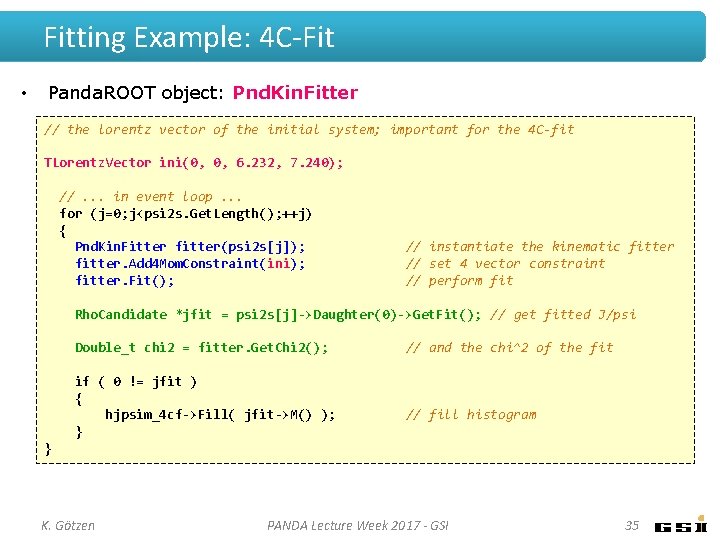
Fitting Example: 4 C-Fit • Panda. ROOT object: Pnd. Kin. Fitter // the lorentz vector of the initial system; important for the 4 C-fit TLorentz. Vector ini(0, 0, 6. 232, 7. 240); //. . . in event loop. . . for (j=0; j<psi 2 s. Get. Length(); ++j) { Pnd. Kin. Fitter fitter(psi 2 s[j]); fitter. Add 4 Mom. Constraint(ini); fitter. Fit(); // instantiate the kinematic fitter // set 4 vector constraint // perform fit Rho. Candidate *jfit = psi 2 s[j]->Daughter(0)->Get. Fit(); // get fitted J/psi Double_t chi 2 = fitter. Get. Chi 2(); if ( 0 != jfit ) { hjpsim_4 cf->Fill( jfit->M() ); } // and the chi^2 of the fit // fill histogram } K. Götzen PANDA Lecture Week 2017 - GSI 35

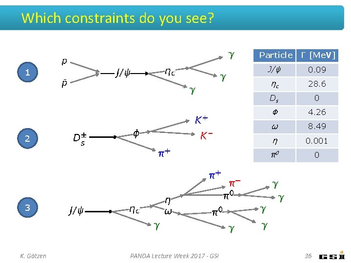
Which constraints do you see? 1 2 Particle Γ [Me. V] J/ψ 0. 09 ηc 28. 6 Ds 0 Φ 4. 26 ω 8. 49 η 0. 001 π0 0 3 K. Götzen PANDA Lecture Week 2017 - GSI 36

UNCERTAINTIES

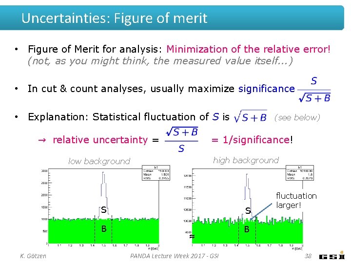
Uncertainties: Figure of merit • Figure of Merit for analysis: Minimization of the relative error! (not, as you might think, the measured value itself. . . ) • In cut & count analyses, usually maximize significance • Explanation: Statistical fluctuation of S is → relative uncertainty = = 1/significance! high background low background K. Götzen (see below) S S B B ≈ PANDA Lecture Week 2017 - GSI fluctuation larger! 38

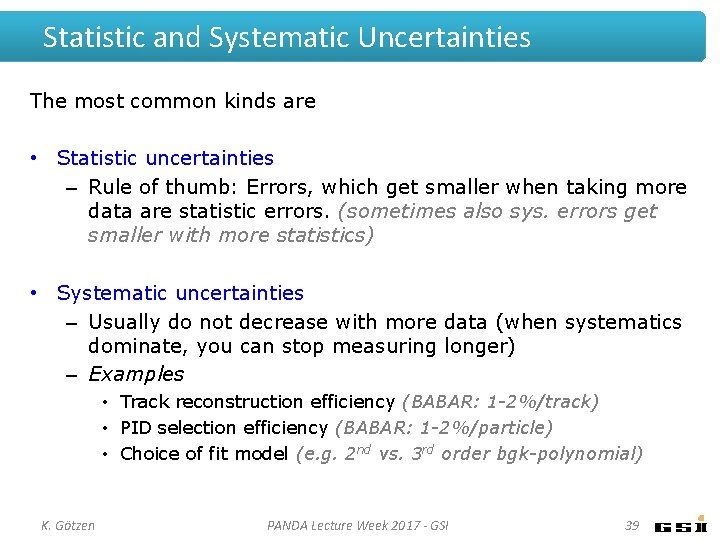
Statistic and Systematic Uncertainties The most common kinds are • Statistic uncertainties – Rule of thumb: Errors, which get smaller when taking more data are statistic errors. (sometimes also sys. errors get smaller with more statistics) • Systematic uncertainties – Usually do not decrease with more data (when systematics dominate, you can stop measuring longer) – Examples • Track reconstruction efficiency (BABAR: 1 -2%/track) • PID selection efficiency (BABAR: 1 -2%/particle) • Choice of fit model (e. g. 2 nd vs. 3 rd order bgk-polynomial) K. Götzen PANDA Lecture Week 2017 - GSI 39

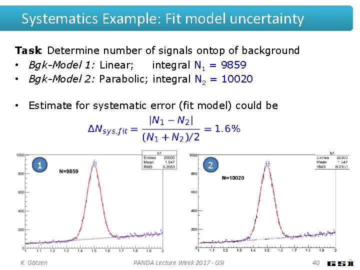
Systematics Example: Fit model uncertainty Task: Determine number of signals ontop of background • Bgk-Model 1: Linear; integral N 1 = 9859 • Bgk-Model 2: Parabolic; integral N 2 = 10020 • Estimate for systematic error (fit model) could be 1 K. Götzen 2 PANDA Lecture Week 2017 - GSI 40

EXERCISES

Exercises Suggestions • Rho Tutorial website: http: //panda-wiki. gsi. de/cgi-bin/view/Computing/Panda. Root. Rho. Tutorial • Take a look to tutorials/thailand 2017/README Exercises: #2 - #6 1. Apply different PID selections and algorithms and compare 2. Apply MC truth match for your reconstructed channels 3. Try different fitters/constraints and compare resolution K. Götzen PANDA Lecture Week 2017 - GSI 42

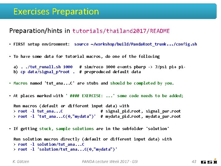
Exercises Preparation/hints in tutorials/thailand 2017/README • FIRST setup environment: source ~/workshop/build/Panda. Root_trunk. . . /config. sh • To have some data for tutorial macros, do one of the following a). . /tut_runall. sh 1000 b) cp data/signal_p*root. # sim/reco 1000 events pbarp -> J/psi pi+ pi# preproduced default data • Macros named 'tut_ana. . . C' are stubs and should be completed by you. • At places marked with ' #### EXERCISE: . . . ' some code needs to be added; Run macros (default or different input data) with > root -l tut_ana. . . C # signal_pid. root, signal_par. root > root -l 'tut_ana. . . C(0, "mydata")' # mydata_pid. root, mydata_par. root • If getting stuck, sample solutions are in the subfolder 'solution' Run solution macros directly (default or different input data) with > root -l solution/tut_ana. . . C > root -l 'solution/tut_ana. . . C(0, "mydata")' K. Götzen PANDA Lecture Week 2017 - GSI 43