Phylogenetic networks Dr Steven Kelk Maastricht University Liege

Phylogenetic networks Dr. Steven Kelk Maastricht University Liege, November 2013

Recommended reading… • Throughout this presentation I refer several times to “Luay’s chapter”. This is a book chapter that appeared a couple of years ago and which is an excellent introduction to this topic: • Nakhleh, Luay. "Evolutionary phylogenetic networks: models and issues. " Problem Solving Handbook in Computational Biology and Bioinformatics. Springer US, 2011. 125 -158.

Gene trees, species trees • As you have heard from Ronald a genome comprises of many genes, organized linearly along the genome. The human genome has about 20, 000. … Gene 1 Gene 2 Gene 3 • The traditional practice in phylogenetics is to construct one phylogenetic tree per gene: a gene tree. (Partly due to the fact that, until relatively recently, we only had information about isolated genes).

Gene trees, species trees • Toy example: four species {dog, cat, fish, e. coli}. We would traditionally identify a gene common to all four (e. g. Gene 1), sequence it, and build a phylogenetic tree for that gene. … Gene 1 Gene 2 Gene 3 • Until relatively recently it was assumed that the gene trees would have the same shape as the species tree.

Gene trees, species trees • The “classical” assumption: … Gene 1 Gene 2 Gene 3 Species tree (same as gene trees)

Gene trees, species trees • However, as more data has become available, and more genes are being sequenced, it has become apparent that in some cases the gene trees can differ from each other, and from the species phylogeny. • The phenomenon of topologically distinct gene trees is called “discordance” or “incongruence”. • But what does this mean? • How can there be multiple evolutionary scenarios for different parts of the genome? • Is the classical assumption of tree-like species evolution wrong?

Gene trees, species trees • What we now sometimes see: … Gene 1 Gene 2 Gene 3 Three distinct gene trees! So what is the species tree? Can we even say there is a species “tree”?

One tree to rule them all…? • There is nothing wrong with the idea of tree-like evolution. • What is wrong with the classical view of evolution, is that there is a single tree that can simultaneously explain everything, in all cases. • The reality is more complex. There are often multiple conflicting tree signals involved. • There actually many different evolutionary phenomena that can cause multiple conflicting tree signals to arise.

So what? • If you feed tree-building software DNA data that actually contains multiple distinct tree signals, it will still produce a single tree for you. But this tree can be (very) misleading. • Sometimes there are clues about this: • Algorithms build very badly supported trees • Extra knowledge about the underlying evolutionary mechanisms • But in general it is extremely easy to confuse nontreelike evolution with a noisy tree signal

Why might we get weak support for a tree? “Noisy tree” Data does fit a single tree, weak support is only a consequence of “noise” “Trees in trees” Data consists of multiple different tree signals…but both gene and species evolution are still ultimately treelike (e. g. due to incomplete lineage sorting, gene loss, gene duplication) “Trees in networks” Data consists of multiple different tree signals…gene evolution is treelike, but species evolution is no longer treelike (e. g. hybridization, horizontal gene transfer) (Note that more microscale evolutionary phenomena, such as recombination, also fall into this category).

Why might we get weak support for a tree? “Noisy tree” Data does fit a single tree, weak support is only a consequence of “noise” “Trees in trees” Data consists of multiple different tree signals…but both gene and species evolution are still ultimately treelike (e. g. due to incomplete lineage sorting, gene loss, gene duplication) “Trees in networks” Data consists of multiple different tree signals…gene evolution is treelike, but species evolution is no longer treelike (e. g. hybridization, horizontal gene transfer) (Note that more microscale evolutionary phenomena, such as recombination, also fall into this category). “RETICULATION”

Very briefly: trees in trees… Here the gene tree (black) is ‘twisted’ inside the species tree (green). In this way many distinct gene trees can be ‘packed’ inside a single species tree. From: L. Nakhleh, "Evolutionary phylogenetic networks: models and issues. " In: The Problem Solving Handbook for Computational Biology and Bioinformatics, L. Heath and N. Ramakrishnan (editors). Springer, 125 -158, 2010.

Trees in networks • For the rest of the lecture I’ll focus on “trees in networks”, which is the situation that occurs due to genuinely reticulate evolutionary phenomena (horizontal gene transfer, hybridization, recombination. . . ) • As Luay’s book chapter explains, distinguishing between “trees in trees” and “trees in networks” (i. e. answering the question: is the species evolution a tree or something more complicated? ) is a major topic of ongoing research. I won’t go into this today.

Phylogenetic networks: 2 types “Data display” / unrooted networks No explicit model of evolution: tries to graphically represent where the data is non-treelike. Does not generate a hypothesis of “what happened”. Evolutionary / rooted /explicit networks Tries to model the events that caused the data to be non-treelike. Tries – in some limited way – to generate a hypothesis of “what happened”.

Phylogenetic networks: 2 types This is what Luay’s book chapter is about. It’s also what I research, so I will almost entirely focus on these types today (rather than data-display networks). Evolutionary / rooted /explicit networks Tries to model the events that caused the data to be non-treelike. Tries – in some limited way – to generate a hypothesis of “what happened”.

Briefly: data-display networks • Mathematically (for me…) not that interesting, but in practice this type of phylogenetic network is still used far more than evolutionary phylogenetic networks. • Why? Because they let the biologist explore the data, and to draw his/her own conclusions. They do not impose a (probably controversial) hypothesis on the biologist. • The following example is from Primer of Phylogenetic Networks by David Morrison: �http: //acacia. atspace. eu/Tutorial. html

Briefly: data-display networks

Briefly: data-display networks This is NOT a hypothesis of evolution!

Briefly: data-display networks • The network on the previous page simultaneously shows multiple bipartitions (“splits”) of the input data. • Each parallel set of edges, when removed, induces such a split. • Where do these splits come from? • DNA data where, per site, at most two different character states are observed (ranging across the species), can be used for this.

Briefly: data-display networks In each of the 43 DNA sites, at most two different DNA characters are observed. So each site induces a bipartition. In this way, there are 9 different bipartitions possible, shown below. (Note that the original numbering of the DNA sites is lost in the figure below). Each parallel set of edges in the network, represents one of these 9 bipartitions.

Briefly: data-display networks

Briefly: data-display networks

Briefly: data-display networks

Evolutionary phylogenetic networks • Used to explicitly model reticulate evolution: • Hybridization • Horizontal Gene Transfer (HGT) • Recombination • Reticulation events have an explicit biological interpretation • Usually rooted, with an explicit “direction” of evolution • Underlying mathematical abstractions are often similar, despite different scale levels of interpretation

Evolutionary phylogenetic networks • Used to explicitly model reticulate evolution: • Hybridization • Horizontal Gene Transfer (HGT) • Recombination • Reticulation events have an explicit biological interpretation • Usually rooted, with an explicit “direction” of evolution • Underlying mathematical abstractions are often similar, despite different scale levels of interpretation “reticulation” or “hybridization” vertices

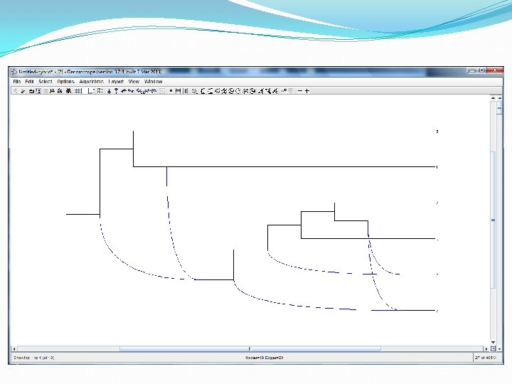
Evolutionary phylogenetic networks In the software package Dendroscope they are drawn left-to-right like this. The point at which two blue lines come together, is a hybridization vertex. This network has a lot of hybridization vertices!

Evolutionary phylogenetic networks In the software package Dendroscope they are drawn left-to-right like this. The point at which two blue lines come together, is a hybridization vertex. This network has a lot of hybridization vertices!

Roadmap… • In the rest of the lecture I am going to discuss two optimization criteria: • Minimum Hybridization • (small) Maximum Parsimony • Both these optimization criteria are based on the idea of “the trees inside the network”. This is exactly the same idea as Luay discusses in his chapter. • “Displays” or “induces” is often used instead of “inside”. But what does it mean?

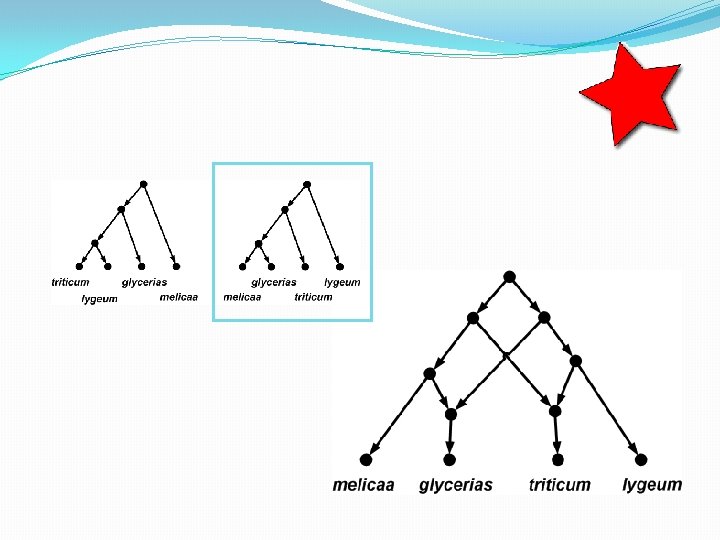
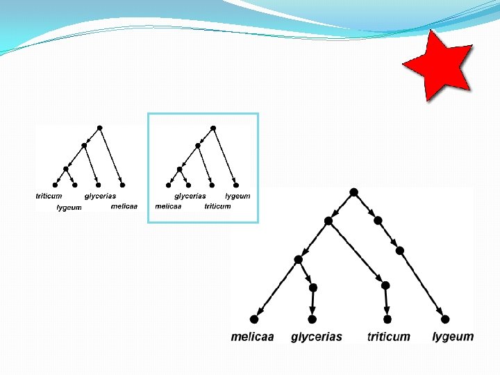
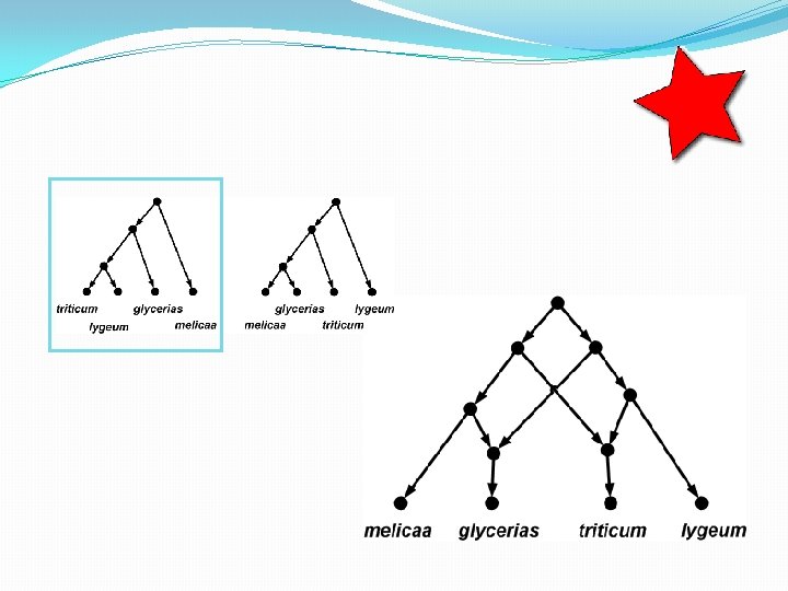
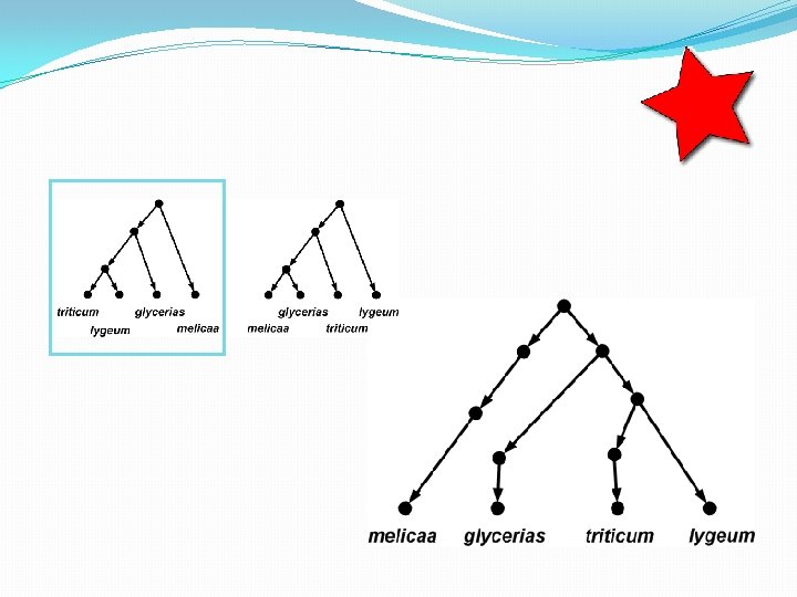
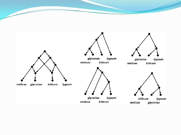
The trees inside…

The trees inside…

How many trees in a network? • A phylogenetic network with r hybridization vertices can display at most 2 r distinct trees. • To see this, observe that for each hybridization vertex you need to delete exactly 1 of its 2 incoming edges. So there are up to 2 r different ways of doing this. • Some of the trees might be the same, however.

A natural goal • Of course, we don’t know what the phylogenetic network looks like. That’s what we want to construct. • In practice we have some of “the trees inside” (gene trees) and we want to infer the phylogenetic network (i. e. species network) that contained them. • “In fact this problem is the holy grail of reticulate evolution. ”

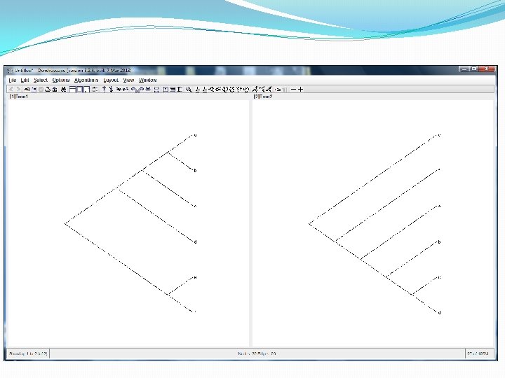
Input: some subset of the trees in the network

Output: the network Input: some subset of the trees in the network

A natural goal • Ideally we want the “true” phylogenetic network. But our (biological) understanding of what this actually means, is still limited, and is a major topic of ongoing research. • I study a very simple mathematical variant, based on Occam’s Razor i. e. preference for simple solutions.

Minimum Hybridization • And this about as simple as it gets… • Input: A set T of (bifurcating) trees, all on the same set of species X. • Output: A phylogenetic network that displays all the input trees whilst minimizing the number of hybridization vertices.

Minimum Hybridization • And this about as simple as it gets… • Input: A set T of (bifurcating) trees, all on the same set of species X. • Output: A phylogenetic network that displays all the input trees whilst minimizing the number of hybridization vertices. • Unfortunately this is already NP-hard for |T|=2

Minimum Hybridization • However, there is NP-hard, and there is NP-hard… • Due to its special underlying combinatorial structure, which we can exploit, we have algorithms that can solve the |T|=2 case for up to 60 hybridizations. • There are many different software packages for this. • Dendroscope contains a competitive algorithm (Algorithms -> Hybridization Networks) , although it is no longer the fastest; this is probably the software package Ultra. Net (2013).

Minimum Hybridization • Why is the |T|=2 case comparatively tractable? • This is because of a mathematical abstraction called the Maximum Acyclic Agreement Forest (MAAF). • The MAAF abstraction allows us to solve the problem without searching through the space of all phylogenetic networks, which is enormous.

Maximum Acyclic Agreement Forests (MAAFs) (This example from Bordewich and Semple 2007) This is an Acyclic Agreement Forest with 4 components.

Minimum Hybridization • We know how to efficiently construct MAAFs, that’s why we can solve the two-tree problem well. • Unfortunately MAAFs don’t “work” for 3 or more trees, this is ongoing research. • That’s enough about Minimum Hybridization. • One more topic to go…MAXIMUM PARSIMONY.

Species 1 (DOG) T G C 2 (CAT) T A C 3 (FISH) A G G 4 (E. COLI) A A G Input: a multiple alignment, one DNA string per species The “most parsimonious” tree solution (4 mutations). An algorithm that computes optimal solutions to MP, will output this tree. From: http: //artedi. ebc. uu. se/course/X 3 -2004/Phylogeny/Exercises/mp. html

Maximum Parsimony (MP) MP classically splits out into two problems: � � “Small” parsimony: � Input: A tree T with its leaves labelled by DNA sequences � Output: A labelling of the interior nodes of the tree, such that the total parsimony score is minimized. “Big” parsimony: � Input: A set of DNA sequences, one per species � Output: The tree T and a labelling of the interior nodes of the tree T, such that the total parsimony score is minimized. So the small problem is calculating the minimum parsimony score for a given tree topology, and the big problem is finding the tree with the minimum such value, ranging over all possible tree topologies.

Maximum Parsimony (MP) That’s all about trees. What about MP on networks? MP classically splits out into two problems: � � “Small” parsimony: � Input: A tree T with its leaves labelled by DNA sequences � Output: A labelling of the interior nodes of the tree, such that the total parsimony score is minimized. “Big” parsimony: � Input: A set of DNA sequences, one per species � Output: The tree T and a labelling of the interior nodes of the tree T, such that the total parsimony score is minimized. So the small problem is calculating the minimum parsimony score for a given tree topology, and the big problem is finding the tree with the minimum such value, ranging over all possible tree topologies.

Maximum Parsimony • We have just seen the Maximum Parsimony (MP) problem on trees, which splits into a small and a big variant. The small variant is easy, using Fitch’s algorithm, the big variant is (NP-)hard. • We can also adapt MP for networks. • How should MP on networks be defined? Do the small and big variants have the same complexity as the tree version of MP?

Maximum Parsimony • Today I will discuss the “softwired” (as opposed to “hardwired”) version of MP on networks. • This is the definition given in Luay’s chapter, and also the one we spend most attention on in the following article: • ON COMPUTING THE MAXIMUM PARSIMONY SCORE OF A PHYLOGENETIC NETWORK, Fischer, Van Iersel, Kelk, Scornavacca (2013).

Maximum Parsimony • The small parsimony problem for networks is quite natural, and defined in terms of “the trees inside”: • The parsimony score of a given network N is equal to the minimum parsimony score ranging over all trees T displayed by N. • So a naïve way to solve the small parsimony problem on networks, would be to loop through all (up to) 2 r trees displayed by the network, use Fitch’s algorithm on each one, and take the minimum. (Just like with trees, you can consider each DNA site separately).

A G

A A G A G A A A G G G

2 2 A G A G 1 G A G A A G G

2 2 A G A G 1 G A G A A G G The lowest-scoring tree has a parsimony score of 1. So the parsimony score of the network (for this DNA string) is 1.

Maximum Parsimony • If the DNA string contains more than 1 site, you can solve for each site separately and sum/combine. • This allows each DNA site to choose its “favourite” tree in the network, independently of the others. • From a modelling perspective this is both a strength and a weakness (too liberal). • In any case: just solving the small parsimony problem on a network is, from a computational perspective, extremely hard (NP-hard and inapproximable). Compare this with trees, where it is very easy…

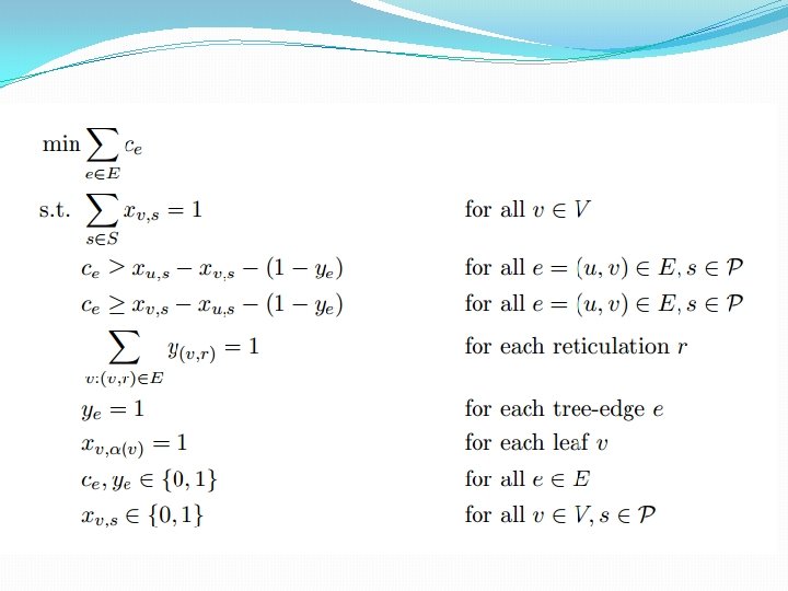
Maximum Parsimony • Fortunately we have shown that the small parsimony problem on networks can be solved quite well in practice using Integer Linear Programming (ILP). • The ILP is part of our software MPNet, downloadable from the internet. • The ILP is shown on the next slide. Don’t worry if you don’t understand what it means.

Output of MPNet for a large network. Red edges are where mutations are incurred on an edge. Blue edges are edges feeding into hybridizations.

Big parsimony…? • Of course, just as the essence of solving MP on trees is finding the best tree (i. e. “big” parsimony), for MP on networks we want to find the best network. • There’s a weird catch though: • Adding hybridizations to a network can allow you to arbitrarily improve the parsimony score. So you have to first limit the number of hybridizations to have a “sensible” problem. • But even when you bound the search space to networks with a small number of hybridizations, the problem is insanely hard: there are so many networks! It’s at least as hard as the big parsimony problem on trees.

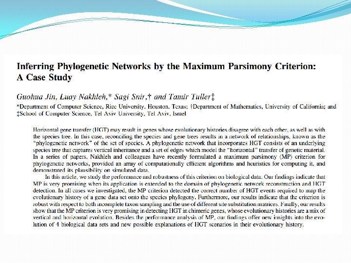
Big parsimony…? • There has been some preliminary work on solving the big parsimony problem for very small datasets, see our ON COMPUTING THE MAXIMUM PARSIMONY SCORE OF A PHYLOGENETIC NETWORK article for a literature survey. • It remains a challenge to balance computational tractability with biological relevance. Lots of work to do here. A notable case study that was undertaken a few years ago:

(HGT edge ≈ hybridization vertex).

That’s it… • I’ve tried to give you a very quick tour through the world of phylogenetic networks. • Of course, it’s only a snapshot of a very large and exciting field, and is biased towards my own (combinatorial) mathematical preferences/prejudices • I hope you’ve enjoyed it. Don’t hesitate to get in touch if you have any questions. • http: //skelk. sdf-eu. org

http: //www 2. lirmm. fr/~gambette/Phylogenetic. Networks/ Shameless propaganda.