Part 6 Market Power 2006 Thomson LearningSouthWestern Chapter

Part 6 Market Power © 2006 Thomson Learning/South-Western

Chapter 13 Monopoly © 2006 Thomson Learning/South-Western

Causes of Monopoly n Barriers to Entry n Technical Barriers to Entry n n 3 Natural Monopoly Legal Barriers to Entry

Profit Maximization n n To maximize profits, a monopoly will chose the output at which marginal revenue equals marginal costs. The demand curve is downward-sloping so marginal revenue is less than price. n 4 To sell more, the firm must lower its price on all units to be sold in order to generate the extra demand.

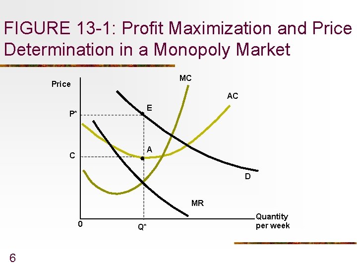
A Graphic Treatment n n A monopoly will produce an output level in which price exceeds marginal cost. Q* is the profit maximizing output level in Figure 13 -1. n 5 If a firm produced less than Q*, the loss in revenue (MR) will exceed the reduction in costs (MC) so profits would decline.

FIGURE 13 -1: Profit Maximization and Price Determination in a Monopoly Market MC Price AC E P* A C D MR 0 6 Q* Quantity per week

A Graphical Treatment n n 7 The increase in costs (MC)would exceed the gain in revenue (MR) if output exceeds Q*. Hence, profits are maximized when MR = MC. Given output level Q*, the firm chooses P* on the demand curve because that is what consumers are willing to pay for Q*. The market equilibrium is P*, Q*.

Monopoly Supply Curve n n n 8 With a fixed market demand curve, the supply “curve” for a monopoly is the one point where MR = MC (point E in Figure 13 -1. ) If the demand curve shifts, the marginal revenue curve will also shift and a new profit maximizing output will be chosen. Unlike perfect competition, these output, price points do not represent a supply curve.

Monopoly Profits n n Monopoly profits are shown as the area of the rectangle P*EAC in Figure 13 -1. Profits equal (P - AC)Q*, n n 9 If price exceeds average cost at Q* > 0, profits will be positive. Since entry is prohibited, these profits can exits in the long run.

Monopoly Rents n Monopoly rents: profits a monopolist earns in the long run. n These profits are a return to the factor that forms the basis of the monopoly. n n 10 Patent, favorable location, license, etc. . Others might be willing to pay up to the amount of this rent to operate the monopoly to obtain its profits.

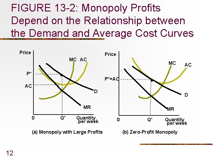
What’s Wrong with Monopoly? n Profitability n n n 11 Monopoly power is the ability to raise price above marginal cost. Profits are the difference between price and average cost. In Figure 13 -2, one firm earns positive economic profits (a) while the other (b) earns zero economic profits.

FIGURE 13 -2: Monopoly Profits Depend on the Relationship between the Demand Average Cost Curves Price MC AC P* P*=AC AC D D MR 0 Q* Quantity per week (a) Monopoly with Large Profits 12 MR 0 Q* Quantity per week (b) Zero-Profit Monopoly

What’s Wrong with Monopoly n Distortion of Resource Allocation n Monopolists restrict their production to maximize profits. n n 13 Since price exceeds marginal cost, consumers are willing to pay more for extra output than it costs to produce it. From societies point of view, output is too low as some mutually beneficial transactions are missed.

Distortion of Resource Allocation n 14 In this situation, a perfectly competitive industry would produce Q* where demand equals long-run supply. A monopolist produces at Q** where marginal revenue equals marginal cost. The restriction in output (Q* - Q**) is a measure of the harm done by a monopoly.

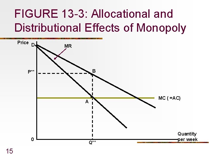
FIGURE 13 -3: Allocational and Distributional Effects of Monopoly Price D MR B P** MC ( =AC) A 0 15 Q** Quantity per week

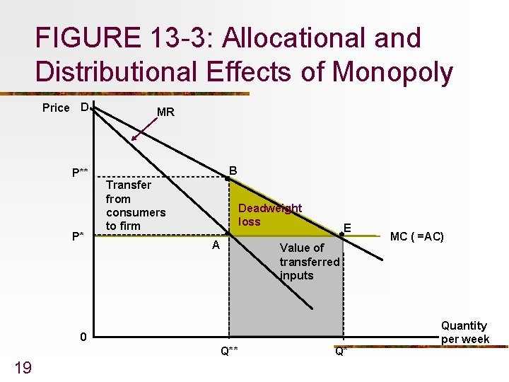
Monopolistic Distortions and Transfers of Welfare n The competitive output level (Q* in Figure 13 -3) is produced at price P*. n n 16 The total value to consumers is the area DEQ*0 Consumers’ pay P*EQ*0. Consumer surplus is DEP*.

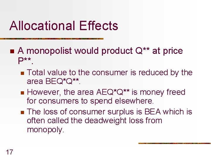
Allocational Effects n A monopolist would product Q** at price P**. n n n 17 Total value to the consumer is reduced by the area BEQ*Q**. However, the area AEQ*Q** is money freed for consumers to spend elsewhere. The loss of consumer surplus is BEA which is often called the deadweight loss from monopoly.

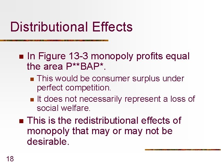
Distributional Effects n In Figure 13 -3 monopoly profits equal the area P**BAP*. n n n 18 This would be consumer surplus under perfect competition. It does not necessarily represent a loss of social welfare. This is the redistributional effects of monopoly that may or may not be desirable.

FIGURE 13 -3: Allocational and Distributional Effects of Monopoly Price D P** P* MR B Transfer from consumers to firm Deadweight loss A E Value of transferred inputs 0 Q** 19 Q* MC ( =AC) Quantity per week

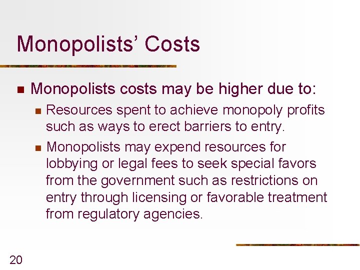
Monopolists’ Costs n Monopolists costs may be higher due to: n n 20 Resources spent to achieve monopoly profits such as ways to erect barriers to entry. Monopolists may expend resources for lobbying or legal fees to seek special favors from the government such as restrictions on entry through licensing or favorable treatment from regulatory agencies.

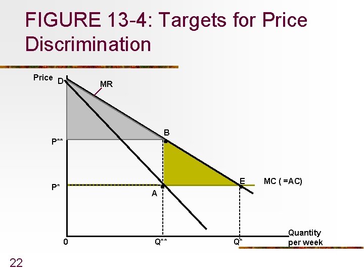
Price Discrimination n n Price discrimination occurs if identical units of output are sold at different prices. If the monopolist could sell its product at different prices to different customers, new opportunities exits as shown in Figure 13 -4. n n 21 Some consumer surplus still exists (area DBP**). The possibility of mutually beneficial trades exist as represented by the area BEA.

FIGURE 13 -4: Targets for Price Discrimination Price D MR B P** E P* A 0 22 MC ( =AC) Q** Q* Quantity per week

Perfect Price Discrimination n Perfect price discrimination is selling each unit of output for the highest price obtainable. n n 23 The firm would sell the first unit at slightly below 0 D (Figure 13 -4), the next for slightly less, and so on until the firm reaches Q*, where a lower price would result in less profit. All consumer surplus (area P*DE) would be monopoly profit.

Perfect Price Discrimination n 24 Since the monopolist would produce and sell Q* units of output, which is the competitive equilibrium. This pricing scheme requires a way to determine what each consumer would be willing to pay, and The monopolist must be able to stop consumers from selling to each other.

Quantity Discounts n Quantity discounts allow some sales at the monopolist’s price (P** in Figure 13 -4), and sales beyond Q** at a lower price which increases profits. n n 25 Examples include a second pizza for a lower price and supermarket coupons. The monopolist must keep customers who buy at lower prices to sell to customers at a price less than P**.

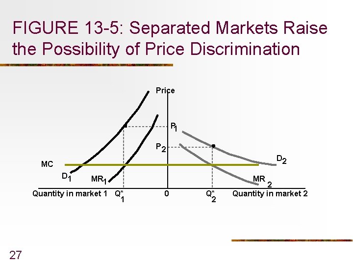
Market Separation n n If the market can be separated into two or more categories may be able to chare different prices. Figure 13 -5 shows the separation into two markets. n 26 The profit-maximizing decision is to sell Q 1* in the first market and Q 2* in the second market where, in both cases, MR = MC.

FIGURE 13 -5: Separated Markets Raise the Possibility of Price Discrimination Price P 1 P 2 D 2 MC D 1 MR 1 Quantity in market 1 Q* 1 27 MR 0 Q* 2 2 Quantity in market 2

Market Separation n The two market prices will be P 1 and P 2 respectively. n n 28 As shown in Figure 13 -5, the pricediscriminating monopolist will charge a higher price in the market with the more inelastic demand. Examples include book publishers charging higher prices in the U. S. or charging different prices for a movie in the day than at night.

Pricing for Multiproduct Monopolies n If a firm has pricing power in markets for several related products, other strategies can be used. n n 29 Firms can require users of one product to also buy a related product such as coffee filters bought with coffee machines. Firms can also create pricing bundles such as option packages on cars or computers.

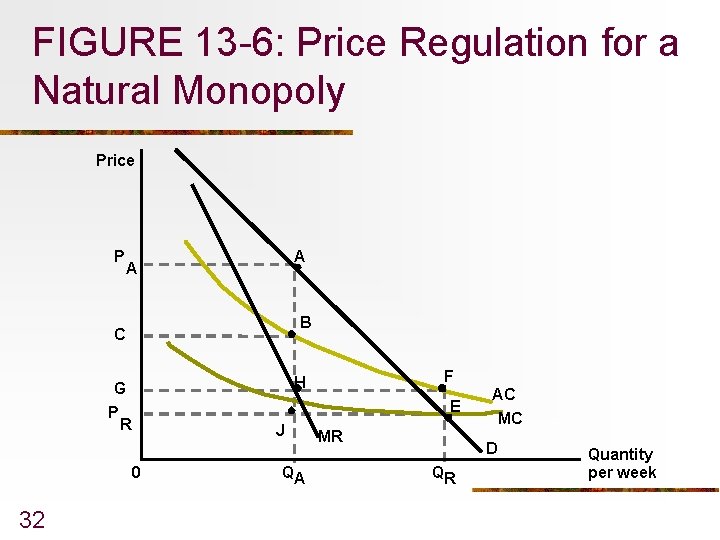
Marginal Cost Pricing Regulation and the Natural Monopoly Dilemma n n By marginal cost pricing the deadweight loss from monopolies is minimized. However, this would require a natural monopoly to operate at a loss. n 30 A unregulated monopoly would produce QA at price PA in Figure 13 -6, yielding a profit of PAABC.

Marginal Cost Pricing Regulation and the Natural Monopoly Dilemma n n 31 Marginal cost pricing of PR which results in QR demanded would generate an a loss equal to the area GFEPR because PR < AC. Either marginal cost pricing must be abandoned or the government must subsidize the monopoly.

FIGURE 13 -6: Price Regulation for a Natural Monopoly Price P A A B C E J 0 32 F H G P R QA MR AC MC D QR Quantity per week

Two-Tier Pricing Systems n n n 33 Under this system the monopoly is permitted to charge some users a high price and charge “marginal” users a low price. The regulatory commission might allow the monopoly to charge PA and sell QA to one class of buyers. Other users would pay PR and would demand QR - Q A.

Two-Tier Pricing Systems n n n 34 At total output of QR average costs are 0 G. Under this system, monopoly profits (area PAAHG) balance the losses (area HFEJ). Here the “marginal user” pays marginal cost and is subsidized by the “intramarginal” user.