Chapter 8 Perfect Competition 2004 Thomson LearningSouthWestern Timing

Chapter 8 Perfect Competition © 2004 Thomson Learning/South-Western

Timing of a Supply Response l l A supply response is the change in quantity of output in response to a change in demand conditions. The pattern of equilibrium prices will be different depending upon the time period – 2 In the very short run, quantity is fixed so there is no supply response

Timing of a Supply Response – – 3 In the short run existing firms may change the quantity they are supplying, but no firms enter or exit the market. In the long run firms can further change the quantity supplied and new firms may enter the market.

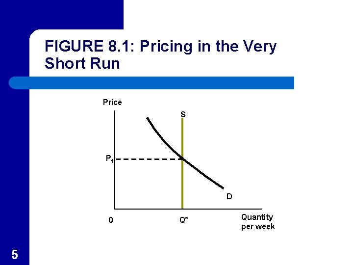
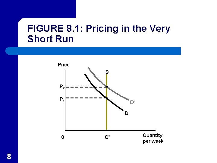
Pricing in the Very Short Run l l l 4 The market period (very short run) is a short period of time during which quantity supplied is fixed. In this period, price acts to ration demand as it adjusts to clear the market. This situation is illustrated in Figure 8. 1 where supply is fixed at Q*.

FIGURE 8. 1: Pricing in the Very Short Run Price S P 1 D 0 5 Q* Quantity per week

Pricing in the Very Short Run l l 6 When demand is represented by the curve D, P 1 is the equilibrium price. The equilibrium price is the price at which the quantity demanded by buyers of a good is equal to the quantity supplied by sellers of the good.

Shifts in Demand: Price as a Rationing Device l l 7 If demand were to increase, as illustrated by the new demand curve D’ in Figure 8. 1, P 1 is no longer the equilibrium price since the quantity demanded exceeds the quantity supplied. The new equilibrium price is now P 2 where price has rationed the good to those who value it the most.

FIGURE 8. 1: Pricing in the Very Short Run Price S P 2 P 1 D’ D 0 8 Q* Quantity per week

APPLICATION 8. 1: Internet Auctions l l l 9 Auctions on the internet have rapidly become one of the most popular ways of selling all manner of goods. There is a sense that internet auctions resemble theoretical situation illustrated in Figure 8. 1…the goods are in fixed supply and will be sold for whatever bidders are willing to pay. However, this view of things may be too simple because it ignores dynamic elements which may be present in suppliers’ decisions.

APPLICATION 8. 1: Internet Auctions l l l 10 A quick examination of internet auction sites suggests that operators employ a variety of features in their auctions. “Reserve” prices, bidding history, and “buy it now” prices are all features offered at various sites. Attempts to answer the many questions that surround the returns to operators usually focus on the uncertainties inherent in the auction process and how bidders respond to them.

APPLICATION 8. 1: Internet Auctions l l l 11 Because buyers and sellers are total strangers in internet auctions, a number of special provisions have been developed to mitigate the risks of fraud that the parties might encounter in such situations. The primary risk facing bidders is in knowing that the goods being offered meet expected quality standards. Previous bidders provide rankings to many of the auction sites.

APPLICATION 8. 1: Internet Auctions l l 12 For sellers, the primary risk is that they will not be paid. Various intermediaries (such as Pay Pal) have been developed to address this problem.

Applicability of the Very Short-Run Model l l This model may only apply where the goods are very perishable. It is usually assumed that a rise in price will prompt producers to bring additional quantity to the market. – 13 This can result from greater production, or, if the goods are durable, from existing stock held by producers.

Short-Run Supply l l l 14 In the short-run the number of firms is fixed as no firms are able to enter or leave the market. However, existing firms can adjust their quantity in response to price changes. Because of the large number of firms, each firm is treated as a price taker.

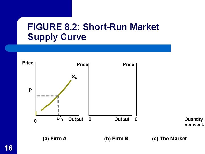
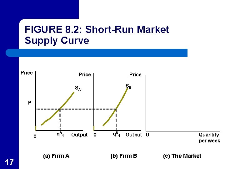
Construction of a Short-Run Supply Curve l l l 15 The quantity that is supplied is the sum of the quantities supplied by each firm. The short-run market supply curve is the relationship between market price and quantity supplied of a good in the short run. In Figure 8. 2 it is assumed that there are only two firms, A and B.

FIGURE 8. 2: Short-Run Market Supply Curve Price SA P 0 q A 1 (a) Firm A 16 Output 0 Output (b) Firm B 0 Quantity per week (c) The Market

FIGURE 8. 2: Short-Run Market Supply Curve Price SB SA P 0 17 q A 1 (a) Firm A Output 0 q B 1 Output 0 (b) Firm B Quantity per week (c) The Market

FIGURE 8. 2: Short-Run Market Supply Curve Price SB SA S P 0 18 q A 1 (a) Firm A Output 0 q B 1 Output 0 (b) Firm B Q 1 Quantity per week (c) The Market

Construction of a Short-Run Supply Curve l l Both firm A’s and firm B’s short-run supply curves (their marginal cost curves) are shown in Figure 8. 2(a) and Figure 8. 2(b) respectively. The market supply curve is the horizontal sum of the two firms are every price. – 19 In Figure 8. 2(c), Q 1 equals the sum of q 1 A and q 1 B.

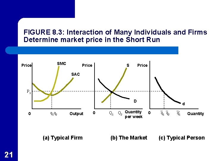
Short-Run Price Determination l l 20 Figure 8. 3 (b) shows the market equilibrium where the market demand curve D and the short-run supply curve S intersect at a price of P 1 and quantity Q 1. This equilibrium would persist since what firms supply at P 1 is exactly what people want to buy at that price.

FIGURE 8. 3: Interaction of Many Individuals and Firms Determine market price in the Short Run Price SMC Price SAC P 1 D 0 q 1 q 2 Output (a) Typical Firm 21 0 Q 1 Q 2 Quantity per week (b) The Market d 0 q 1 q 2 q‘ 1 Quantity (c) Typical Person

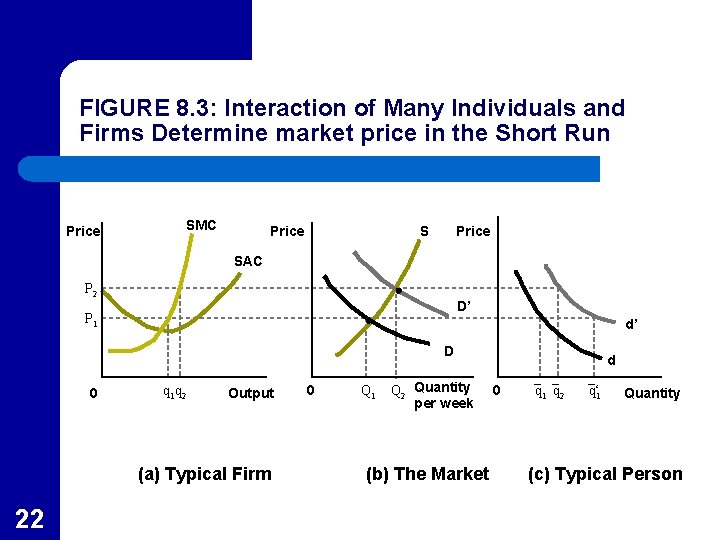
FIGURE 8. 3: Interaction of Many Individuals and Firms Determine market price in the Short Run Price SMC Price SAC P 2 D’ P 1 d’ D 0 q 1 q 2 Output (a) Typical Firm 22 0 Q 1 Q 2 Quantity per week (b) The Market d 0 q 1 q 2 q‘ 1 Quantity (c) Typical Person

Functions of the Equilibrium Price l The price serves as a signal to producers about how much should be produced. – – 23 To maximize profit, firms will produce the output level for which marginal costs equal P 1. This yields an aggregate production of Q 1.

Functions of the Equilibrium Price l Given the price, utility maximizing individuals will decide how much of their limited incomes to spend – – l 24 At price P 1 the total quantity demanded is Q 1. No other price brings about the balance of quantity demanded and quantity supplied. These situations are depicted in Figure 8. 3 (a) and (b) for the typical firm and individual, respectively.

Effect of an Increase in Market Demand l l 25 If the typical person’s demand for the good increases from d to d’, the entire market demand curve will shift to D’ as shown in figure 8. 3. The new equilibrium is P 2, Q 2 where a new balance between demand supply is established.

Effect of an Increase in Market Demand l l l 26 The increase in demand resulted in a higher equilibrium price, P 2 and a greater equilibrium quantity, Q 2. P 2 has rationed the typical person’s demand so that only q 2 is demanded rather than the q’ 1 that would have been demanded at P 1. P 2 also signals the typical firm to increase production from q 1 to q 2.

Shifts in Demand Curves l Demand will increase, shift outward, because – – 27 Income increases The price of a substitute rises The price of a complement falls Preferences for the good increase

Shifts in Demand Curves l Demand will decrease, shift inward, because – – 28 Income falls The price of a substitute falls The price of a complement rises Preferences for the good diminish

Shifts in Supply Curves l Supply will increase, shift outward, because – – l Supply will decrease, shift inward, because – 29 Input prices fall Technology improves Input prices rise

Table 8. 1: Reasons for a Shift in a Demand or Supply Curve 30

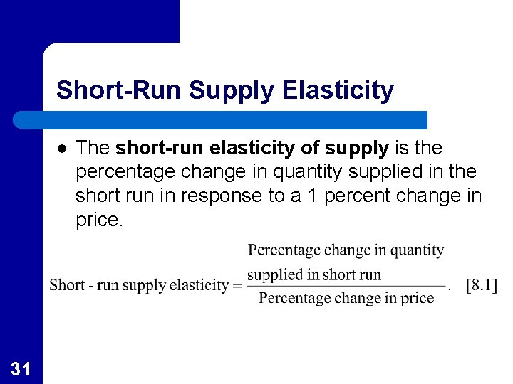
Short-Run Supply Elasticity l 31 The short-run elasticity of supply is the percentage change in quantity supplied in the short run in response to a 1 percent change in price.

Short-Run Supply Elasticity l l 32 If a 1 percent increase in price causes firms to increase quantity supplied by more than 1 percent, supply is elastic. If a 1 percent increase in price causes firms to increase quantity supplied by less than 1 percent, supply is inelastic.

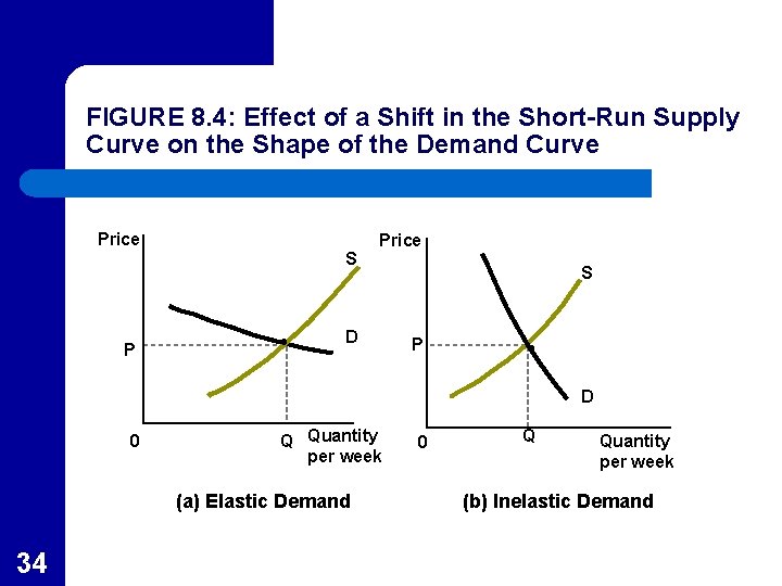
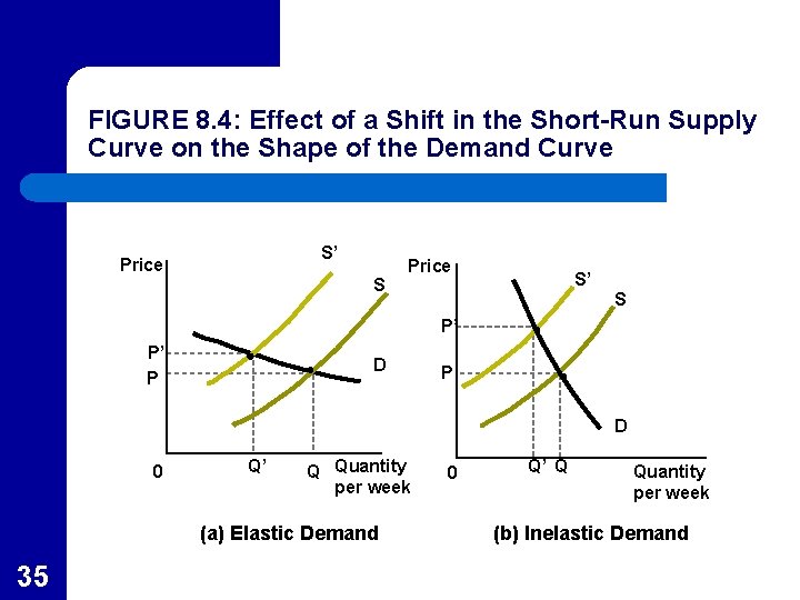
Shits in Supply Curves and the Importance of the Shape of the Demand Curve l The effect of a shift in supply upon equilibrium levels of P and Q depends upon the shape of the demand curve. – – 33 If demand is elastic, as in Figure 8. 4 (a), a decrease in supply has a small effect on price but a relatively large effect on quantity. If demand is inelastic, as in Figure 8. 4 (b), the decrease in supply has a greater effect on price than on quantity.

FIGURE 8. 4: Effect of a Shift in the Short-Run Supply Curve on the Shape of the Demand Curve Price S P Price D S P D 0 Q Quantity per week (a) Elastic Demand 34 0 Q Quantity per week (b) Inelastic Demand

FIGURE 8. 4: Effect of a Shift in the Short-Run Supply Curve on the Shape of the Demand Curve S’ Price S’ S P’ P’ P D 0 Q’ Q Quantity per week (a) Elastic Demand 35 0 Q’ Q Quantity per week (b) Inelastic Demand

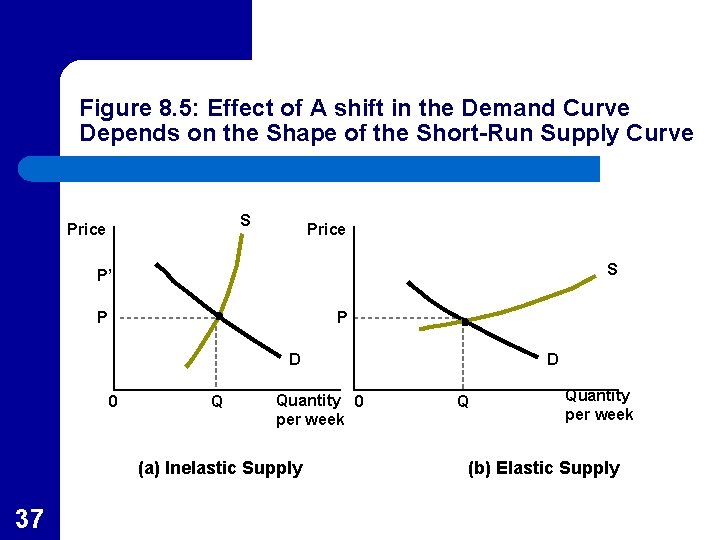
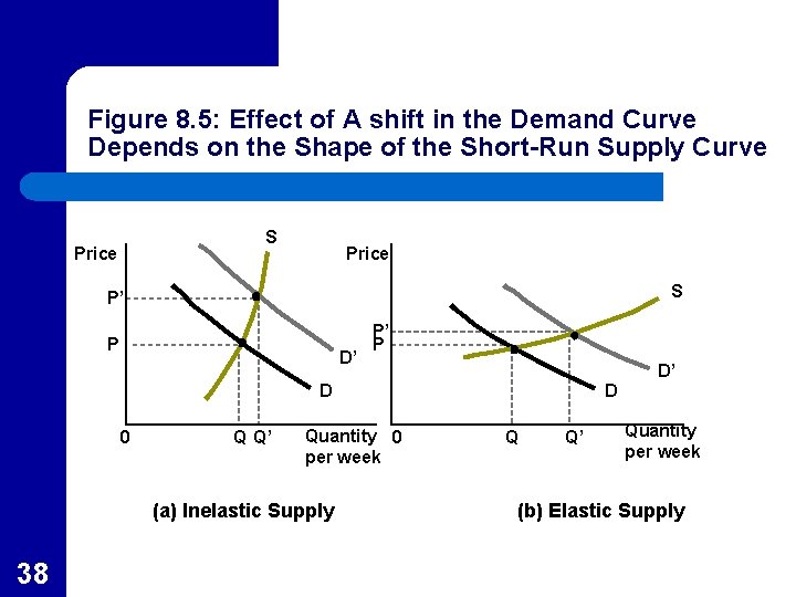
Shifts in Demand Curves and the Importance of the Shape of the Supply Curve l The effect of a shift in demand upon equilibrium levels of P and Q depends upon the shape of the supply curve. – – 36 If supply is inelastic, as in Figure 8. 5 (a), the effect on price is much greater than on quantity. If the supply curve is elastic, as in Figure 8. 5 (b), the effect on price is relatively smaller than the effect on quantity.

Figure 8. 5: Effect of A shift in the Demand Curve Depends on the Shape of the Short-Run Supply Curve S Price S P’ P P D 0 Q Quantity 0 per week (a) Inelastic Supply 37 D Q Quantity per week (b) Elastic Supply

Figure 8. 5: Effect of A shift in the Demand Curve Depends on the Shape of the Short-Run Supply Curve S Price S P’ P D’ D 0 Q Q’ Quantity 0 per week (a) Inelastic Supply 38 D Q Q’ Quantity per week (b) Elastic Supply

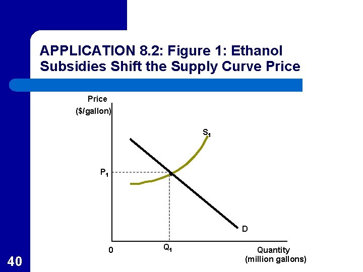
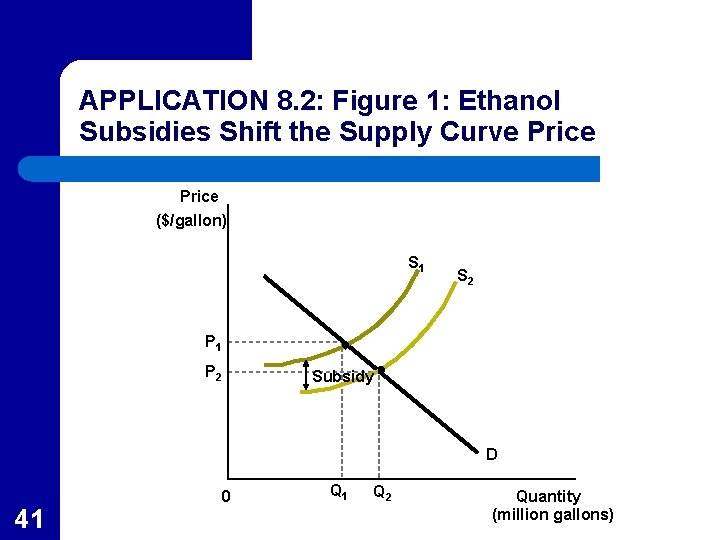
APPLICATION 8. 2: Ethanol Subsidies in the United States and Brazil l 39 Ethanol has potentially desirable properties as a fuel for automobiles or additive to gasoline that may reduce air pollution. Several governments have adopted subsides to producers of ethanol. One way to show the effect of a subsidy is to treat it as a shift in the short-run supply curve as shown in Figure 1.

APPLICATION 8. 2: Figure 1: Ethanol Subsidies Shift the Supply Curve Price ($/gallon) S 1 P 1 D 0 40 Q 1 Quantity (million gallons)

APPLICATION 8. 2: Figure 1: Ethanol Subsidies Shift the Supply Curve Price ($/gallon) S 1 S 2 P 1 P 2 Subsidy D 0 41 Q 2 Quantity (million gallons)

APPLICATION 8. 2: Ethanol Subsidies in the United States and Brazil l l 42 The subsidy shifts out the supply curve (by about 54 cents-a-gallon in the U. S. ) which results in a quantity demanded increase from Q 1 to Q 2. The total cost of the subsidy depends upon the per-gallon amount and on the amount of the increase in quantity demanded.

APPLICATION 8. 2: Ethanol Subsidies in the United States and Brazil l 43 In the U. S. it is made from corn, and the subsidy is primarily found in Iowa where many major corn producers are located. In Brazil it is made from sugar cane and was heavily subsidized until Economic liberalization in the 1990 s. Due to political pressure from producers, the subsidy is again being proposed.

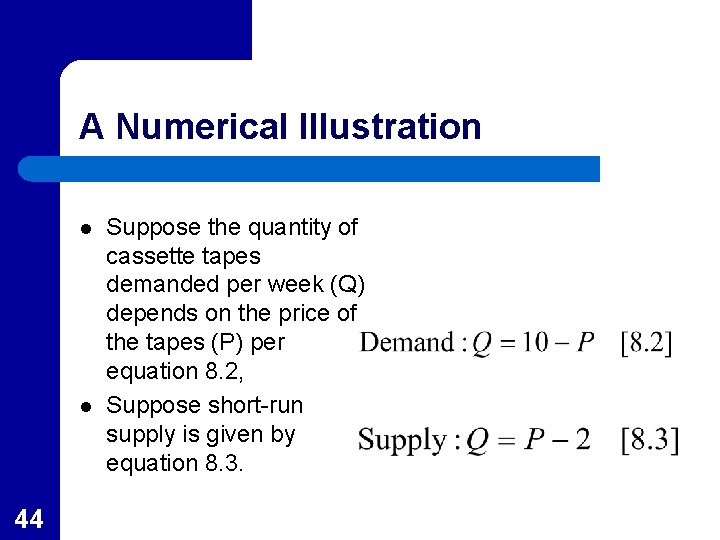
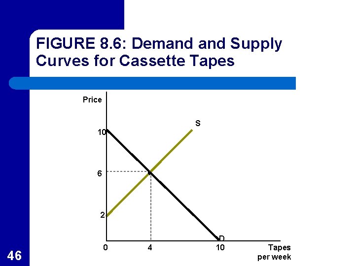
A Numerical Illustration l l 44 Suppose the quantity of cassette tapes demanded per week (Q) depends on the price of the tapes (P) per equation 8. 2, Suppose short-run supply is given by equation 8. 3.

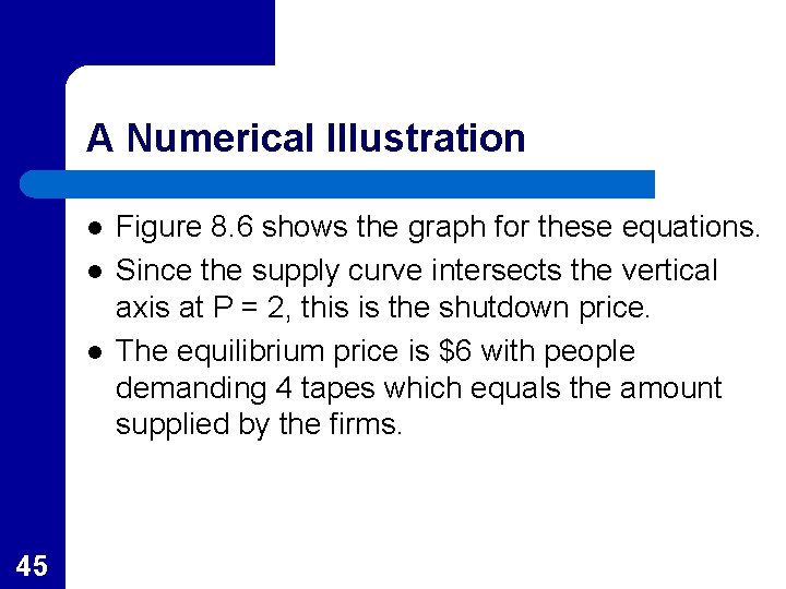
A Numerical Illustration l l l 45 Figure 8. 6 shows the graph for these equations. Since the supply curve intersects the vertical axis at P = 2, this is the shutdown price. The equilibrium price is $6 with people demanding 4 tapes which equals the amount supplied by the firms.

FIGURE 8. 6: Demand Supply Curves for Cassette Tapes Price S 10 6 2 46 0 4 D 10 Tapes per week

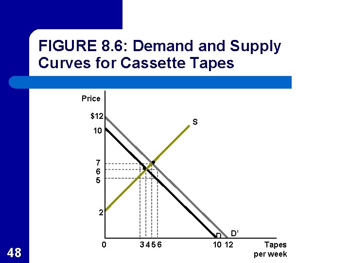
A Numerical Illustration l l 47 If the demand increased as reflected in equation 8. 4, the former equilibrium price and quantity would no longer hold. As shown in Figure 8. 6, the new equilibrium price is $7 where the quantity demanded and supplied of tapes is 5.

FIGURE 8. 6: Demand Supply Curves for Cassette Tapes Price $12 S 10 7 6 5 2 48 0 3456 D D’ 10 12 Tapes per week

A Numerical Illustration l l l 49 Table 8. 2 shows the two cases. After the increase in demand, there is an excess demand for tapes at the old equilibrium price of $6. The increase in price from $6 to $7 restores equilibrium in the market.

TABLE 8. 2: Supply and Demand Equilibrium in the Market for Cassette Tapes 50 New equilibrium Initial equilibrium

The Long Run l Long run supply responses are much more flexible than in the short run. – – 51 Long-run cost curves reflect greater input flexibility. Firms can enter and exit the market in response to profit opportunities.

Equilibrium Conditions l In a perfectly competitive equilibrium, no firm has an incentive to change its behavior. – – 52 Firms must be choosing the profit maximizing level of output. Firms must be content to stay in or out of the market.

Profit Maximization l It is assumed that the goal of each firm is to maximize profits. – – 53 Since each firm is a price taker, this implies that each firm product where price equals long-run marginal cost. This equilibrium condition, P = MC determines the firm’s output choice and its choice of inputs that minimize their long-run costs.

Entry and Exit l The perfectly competitive model assumes that firms entail no special costs when they exit and enter the market. – – 54 Firms will be enticed to enter the market when economic profits are positive. Firms will leave the market when economic profits are negative.

Entry and Exit l Entry will cause the short-run market supply curve to shift outward causing the market price to fall. – l 55 This will continue until positive economic profits are no longer available. Exit causes the short-run market supply curve to shift inward causing the market price to increase, eliminating the economic losses.

Long-Run Equilibrium l l l 56 For purposes of this chapter, it is assumed that all firms producing a particular good have identical cost curves. Thus, in the long-run equilibrium all firms earn zero economic profits. Firms will produce at minimum average total costs where P = MC and P = AC.

Long-Run Equilibrium l l l 57 P = MC results from the assumption that firm’s are profit maximizers. P = AC results because market forces cause long run economic profits to equal zero. In the long run, firm owners will only earn normal returns on their investments.

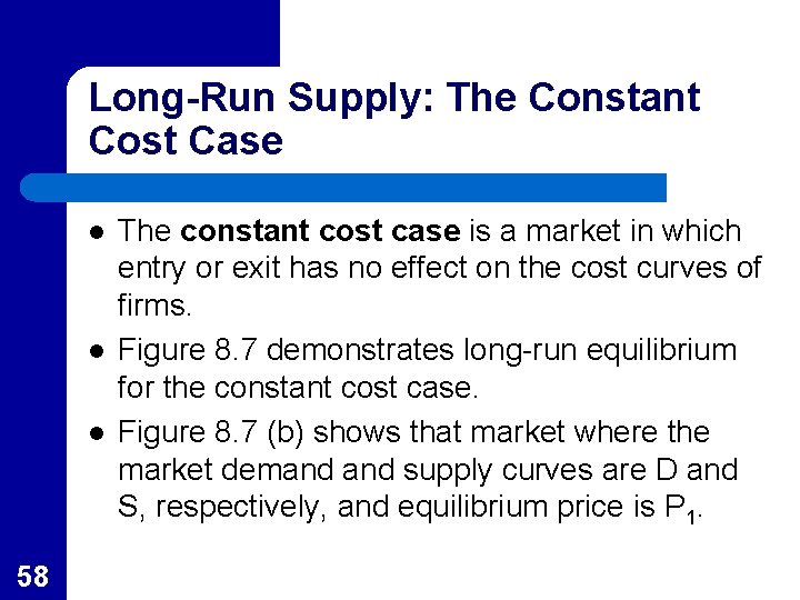
Long-Run Supply: The Constant Cost Case l l l 58 The constant cost case is a market in which entry or exit has no effect on the cost curves of firms. Figure 8. 7 demonstrates long-run equilibrium for the constant cost case. Figure 8. 7 (b) shows that market where the market demand supply curves are D and S, respectively, and equilibrium price is P 1.

FIGURE 8. 7: Long-Run Equilibrium for a Perfectly Competitive Constant Market: Cost Case Price SMC MC S AC P 1 D 0 q 1 (a) Typical Firm 59 Output 0 Q 1 Quantity per week (b) Total Market

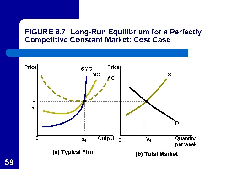
FIGURE 8. 7: Long-Run Equilibrium for a Perfectly Competitive Constant Market: Cost Case Price SMC MC S AC P 2 P 1 D D 0 60 q 1 q 2 (a) Typical Firm Output 0 Q 1 Q 2 Quantity per week (b) Total Market

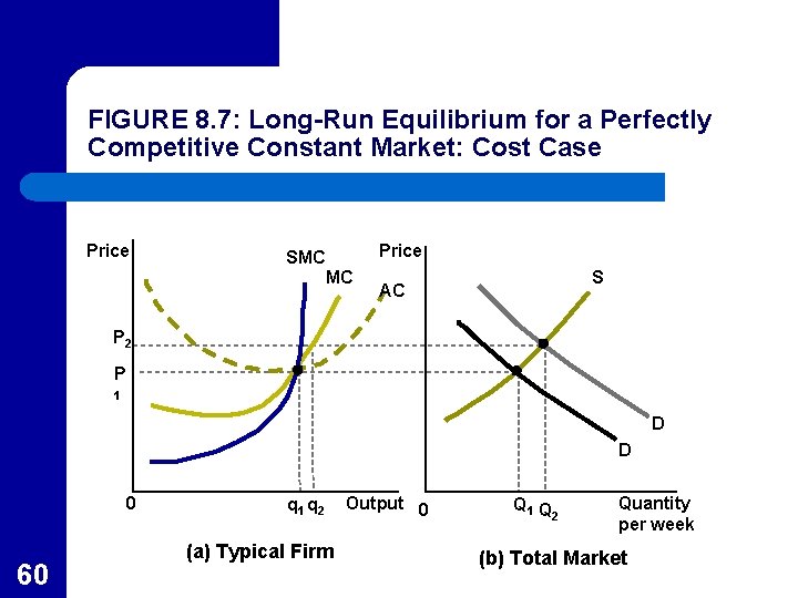
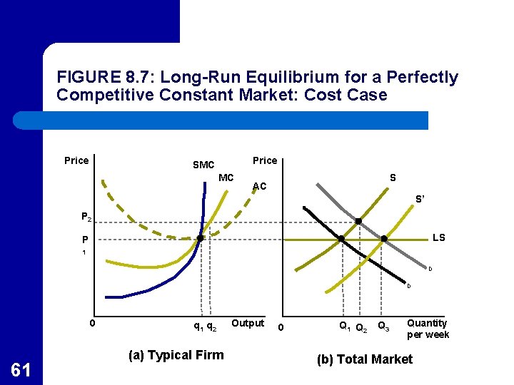
FIGURE 8. 7: Long-Run Equilibrium for a Perfectly Competitive Constant Market: Cost Case Price SMC MC S AC S’ P 2 LS P 1 D D 0 61 q 2 (a) Typical Firm Output 0 Q 1 Q 2 Q 3 Quantity per week (b) Total Market

Long-Run Supply: The Constant Cost Case l l 62 The typical firm will produce output level q 1 which results in Q 1 in the market. The typical firm is maximizing profits since price is equal to long-run marginal cost. The typical firm is earning zero economic profits since price equals long-run average total costs. There is no incentive for exit or entry.

A Shift in Demand l l l 63 If demand increases to D’, the short-run price will increase to P 2. A typical firm will maximize profits by producing q 2 which will result in short-run economic profits (P 2 > AC). Positive economic profits cause new firms to enter the market until economic profits again equal zero.

A Shift in Demand l l l 64 Since costs do no increase with entry, the typical firm’s costs curves do not change. The supply curve shifts to S’ where the equilibrium price returns to P 1 and the typical firm produces q 1 again. The new long-run equilibrium output will be Q 3 with more firms in the market.

Long-Run Supply Curve l l l 65 Regardless of the shift in demand, market forces will cause the equilibrium price to return to P 1 in the long-run. The long-run supply curve is horizontal at the low point of the firms long-run average total cost curves. This long-run supply curve is labeled LS in Figure 8. 7 (b).

APPLICATION 8. 3: Movie Rentals l l 66 Movies have been available for home rental since the 1920 s. The basic rental business has consistently exhibited the characteristics of a constant cost industry. By the end of the 1980 s, more than 70% of U. S. households owned VHS tape players. At first the rental industry was quite profitable, but there were no significant barriers to entry.

APPLICATION 8. 3: Movie Rentals l l 67 Because inputs used by the industry (low-wage workers and simple rental space) were readily available at market prices, the industry had a perfectly elastic long-run supply curve – it could easily meet exploding demand with no increase in price. The number of tape rental outlets grew fourfold and the standard price for rental of a movies fell to about $1. 50 per night.

APPLICATION 8. 3: Movie Rentals l l l 68 Introduction of DVD technology in the mid 1990 s followed a similar path. Once a critical threshold of households owned DVD players, the rental market for movies on DVD emerged quickly. Again, the absence of barriers to entry together with the ready availability of inputs resulted in a close approximation to the constant cost model.

APPLICATION 8. 3: Movie Rentals l l l 69 This elastic supply response has also dictated a strict market test for innovations in the movie rental business – such innovations must be cost-competitive with existing methods of distribution or they will not be adopted. The fate of “Divx” technology provides an instructive example. Because consumers had to purchase special equipment, Divx gained few adherents and was largely abandoned by the start of 1999.

Shape of the Long-Run Supply Curve: The Increasing Cost Case l The increasing cost case is a market in which the entry of firms increases firms’ costs. – – – 70 New firms may increase demand for scarce inputs driving up their prices. New firms may impose external costs in the form of air or water pollution. New firms may place strains on public facilities increasing costs for all firms in the market.

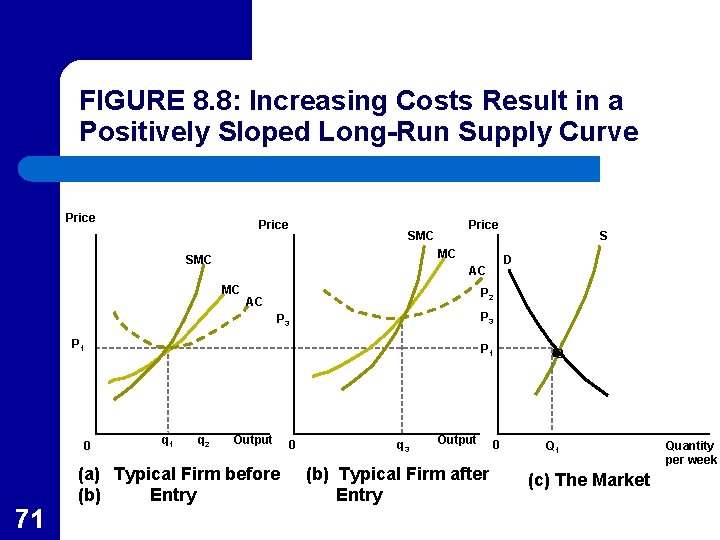
FIGURE 8. 8: Increasing Costs Result in a Positively Sloped Long-Run Supply Curve Price SMC MC SMC P 2 AC P 3 P 1 0 71 D AC MC P 1 q 2 S Output (a) Typical Firm before (b) Entry 0 q 3 Output (b) Typical Firm after Entry 0 2 Q 1 (c) The Market Quantity per week

FIGURE 8. 8: Increasing Costs Result in a Positively Sloped Long-Run Supply Curve Price SMC MC P 2 SMC MC q 1 q 2 Output 0 S D P 1 (a) Typical Firm before Entry 72 AC D’ P 2 AC P 1 0 Price q 3 Output 0 (b) Typical Firm after Entry 2 Q 1 Q 2 Q 3 (c) The Market Quantity per week

FIGURE 8. 8: Increasing Costs Result in a Positively Sloped Long-Run Supply Curve Price SMC MC P 2 AC Price SMC MC D AC P 3 q 2 Output 0 (a) Typical Firm before Entry 73 S’ LS P 3 P 1 q 1 S P 2 P 1 0 D’ q 3 Output 0 (b) Typical Firm after Entry 2 Q 1 Q 2 Q 3 (c) The Market Quantity per week

The Increasing Cost Case l l 74 This case is shown in Figure 8. 8, where the initial equilibrium price is P 1 with the typical firm producing q 1 with total output Q 1. Economic profits are zero. The increase in demand to D’, with short-run supply curve S, causes equilibrium price to increase to P 2 with the typical firm producing q 2 resulting in positive profits.

The Increasing Cost Case l l 75 The positive profits entice firms to enter which drives up costs. The typical firm’s new cost curves are shown in Figure 8. 8 (b). The new long-run equilibrium price is P 3 with market output Q 3. The long-run supply curve, LS, is positively sloped because of the increasing costs.

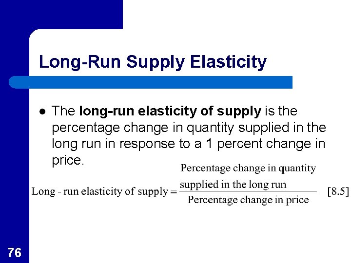
Long-Run Supply Elasticity l 76 The long-run elasticity of supply is the percentage change in quantity supplied in the long run in response to a 1 percent change in price.

TABLE 8. 3: Estimated Long-Run Supply Elasticities 77

The Decreasing Cost Case l The decreasing cost case is a market in which the entry of firms decreases firms’ costs. – – 78 Entry may produce a larger pool of trained labor which reduces the costs of hiring. Entry may provide a “critical mass” of industrialization that permits the development of more efficient transportation, communications, and financial networks.

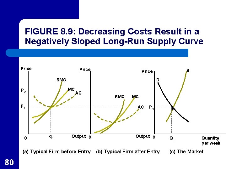
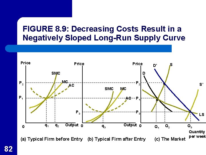
The Decreasing Cost Case l l l 79 The initial equilibrium is shown as P 1, Q 1 in Figure 8. 9 (c). The increase in demand from D to D’ results in the short-run equilibrium, P 2, Q 2 where the typical firm is earning positive economic profits. Entry drives down costs for the typical firm, as shown in Figure 8. 9 (b).

FIGURE 8. 9: Decreasing Costs Result in a Negatively Sloped Long-Run Supply Curve Price SMC D MC P 2 AC P 1 0 Output 0 (a) Typical Firm before Entry 80 SMC MC AC q 1 S Price P 1 Output 0 (b) Typical Firm after Entry 2 Q 1 Quantity per week (c) The Market

FIGURE 8. 9: Decreasing Costs Result in a Negatively Sloped Long-Run Supply Curve Price SMC D MC P 2 AC P 1 0 P 2 SMC MC AC q 1 q 2 Output 0 P 1 Output 0 (a) Typical Firm before Entry (b) Typical Firm after Entry 81 S D’ 2 Q 1 Q 2 Quantity per week (c) The Market

FIGURE 8. 9: Decreasing Costs Result in a Negatively Sloped Long-Run Supply Curve Price SMC D MC P 2 AC SMC P 1 q 2 Output 0 (a) Typical Firm before Entry 82 S’ MC AC P 3 0 S D’ P 1 2 P 3 q 3 Output 0 (b) Typical Firm after Entry LS Q 1 Q 2 (c) The Market Q 3 Quantity per week

The Decreasing Cost Case l l l 83 Entry continues until short-run economic profits are eliminated. The new long-run equilibrium is P 3, Q 3 as shown in Figure 8. 9 (c). The long-run supply curve is downward sloping due to the decreasing costs as labeled LS in Figure 8. 9 (c).

APPLICATION 8. 4: How Do Network Externalities Affect Supply Curves? l Network externalities occur when additional users cause network costs to decline. – 84 Subject to Metcalfe’s Law which states that the number of interconnections possible in a given communications network expands with the square of the number of subscribers in the network.

APPLICATION 8. 4: How Do Network Externalities Affect Supply Curves? l These cause negatively sloped long-run supply curves. – l 85 This can cause lower consumer prices when demand expands. Industries subject to network externalities include telecommunications, computer software, and the Internet.

APPLICATION 8. 4: How Do Network Externalities Affect Supply Curves? l Telecommunications – l Computer Software – – 86 Most of the gains in developed countries have been realized, but remain for less developed. As adoption grows, lower learning costs for users. These benefits may explain why software companies are not too concerned with pirating.

APPLICATION 8. 4: How Do Network Externalities Affect Supply Curves? l The Internet – – 87 Since anything that can be encoded in digital format can be shared over the network, benefits for specialized groups can also be realized. This, along with the improved storage capacity of computers, makes it possible to provide specific types of services that where cost prohibitive before the Internet.

Infant Industries l Initially the cost of production of a new product may be very high. – l 88 As the pool of skilled workers grows, costs may decline. It is often argued that these “infant” industries must be protected from lower-cost foreign competition until they reach the lower cost portion of their supply curves.