Chapter 17 Asymmetric Information 2006 Thomson LearningSouthWestern Asymmetric

Chapter 17 Asymmetric Information © 2006 Thomson Learning/South-Western

Asymmetric Information n 2 In a game with uncertainty, asymmetric information refers to the information that one player has but the other does not.

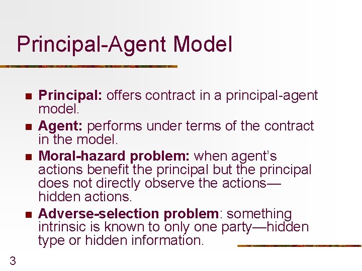
Principal-Agent Model n n 3 Principal: offers contract in a principal-agent model. Agent: performs under terms of the contract in the model. Moral-hazard problem: when agent’s actions benefit the principal but the principal does not directly observe the actions— hidden actions. Adverse-selection problem: something intrinsic is known to only one party—hidden type or hidden information.

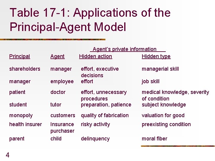
Table 17 -1: Applications of the Principal-Agent Model Principal Agent shareholders manager employee patient doctor student Agent’s private information Hidden action Hidden type effort, executive decisions effort managerial skill tutor effort, unnecessary procedures preparation, patience medical knowledge, severity of condition subject knowledge monopoly customers quality of fabrication valuation for good health insurer Insurance purchaser child risky activity preexisting condition delinquency moral fiber parent 4 job skill

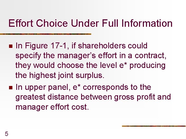
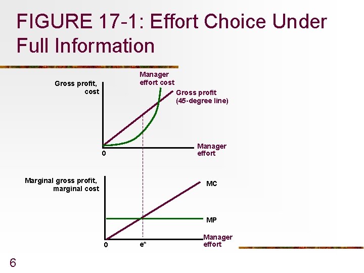
Effort Choice Under Full Information n n 5 In Figure 17 -1, if shareholders could specify the manager’s effort in a contract, they would choose the level e* producing the highest joint surplus. In upper panel, e* corresponds to the greatest distance between gross profit and manager effort cost.

FIGURE 17 -1: Effort Choice Under Full Information Manager effort cost Gross profit, cost Gross profit (45 -degree line) Manager effort 0 Marginal gross profit, marginal cost MC MP 0 6 e* Manager effort

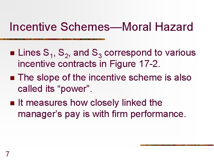
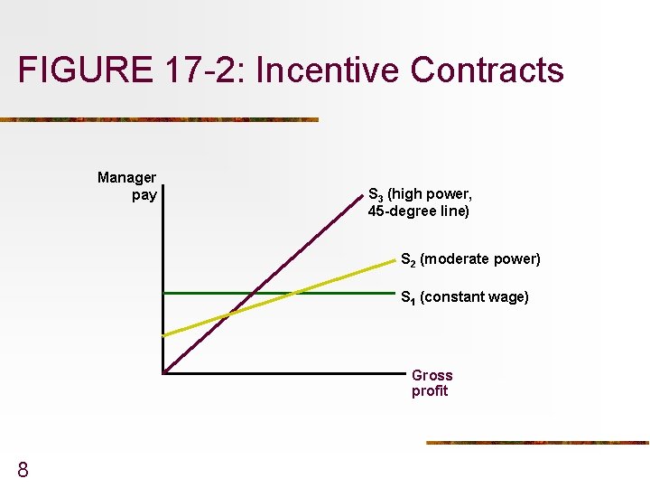
Incentive Schemes—Moral Hazard n n n 7 Lines S 1, S 2, and S 3 correspond to various incentive contracts in Figure 17 -2. The slope of the incentive scheme is also called its “power”. It measures how closely linked the manager’s pay is with firm performance.

FIGURE 17 -2: Incentive Contracts Manager pay S 3 (high power, 45 -degree line) S 2 (moderate power) S 1 (constant wage) Gross profit 8

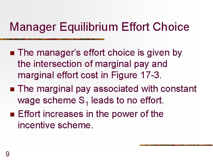
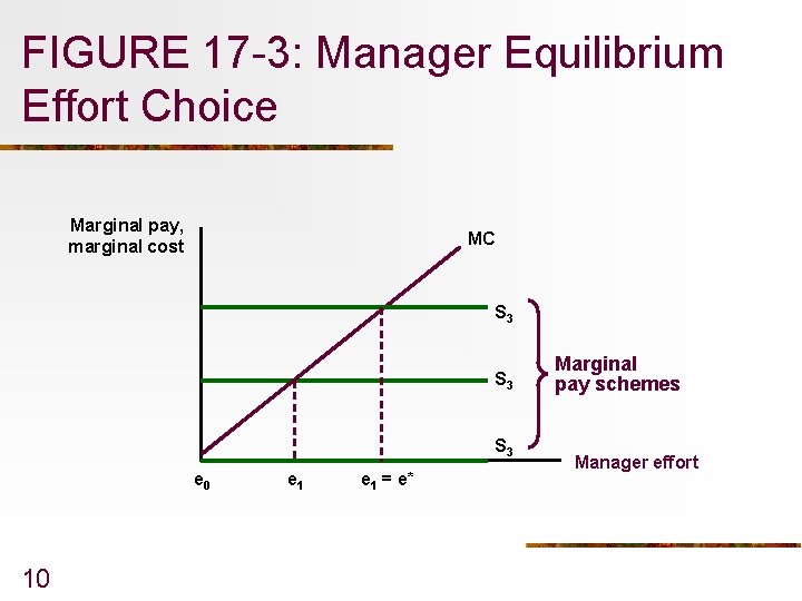
Manager Equilibrium Effort Choice n n n 9 The manager’s effort choice is given by the intersection of marginal pay and marginal effort cost in Figure 17 -3. The marginal pay associated with constant wage scheme S 1 leads to no effort. Effort increases in the power of the incentive scheme.

FIGURE 17 -3: Manager Equilibrium Effort Choice Marginal pay, marginal cost MC S 3 S 3 e 0 10 e 1 = e* Marginal pay schemes Manager effort

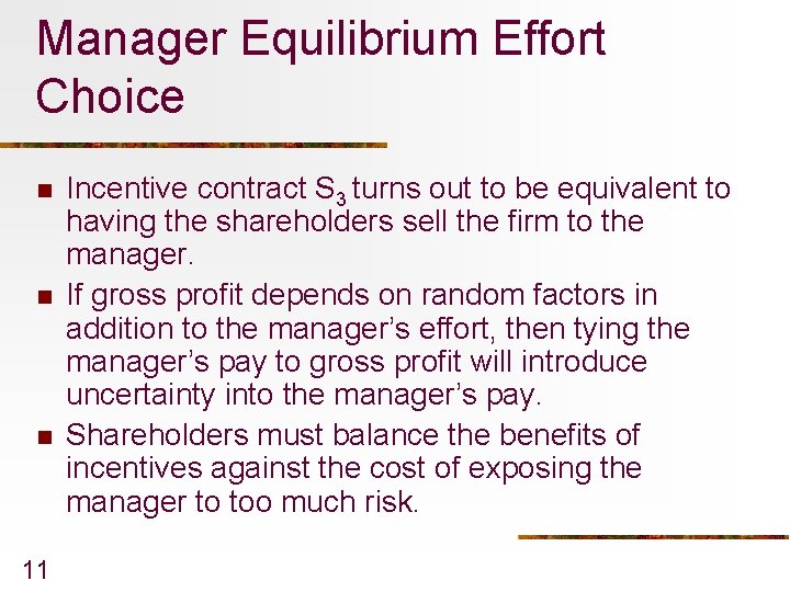
Manager Equilibrium Effort Choice n n n 11 Incentive contract S 3 turns out to be equivalent to having the shareholders sell the firm to the manager. If gross profit depends on random factors in addition to the manager’s effort, then tying the manager’s pay to gross profit will introduce uncertainty into the manager’s pay. Shareholders must balance the benefits of incentives against the cost of exposing the manager to too much risk.

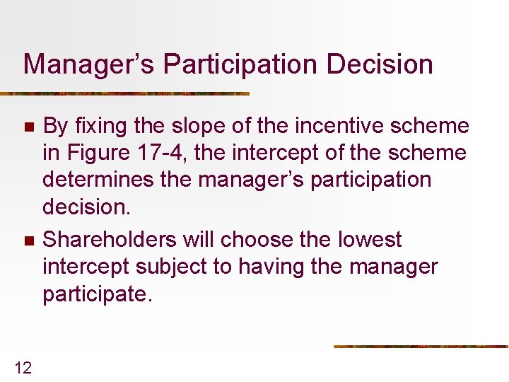
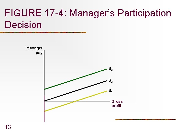
Manager’s Participation Decision n n 12 By fixing the slope of the incentive scheme in Figure 17 -4, the intercept of the scheme determines the manager’s participation decision. Shareholders will choose the lowest intercept subject to having the manager participate.

FIGURE 17 -4: Manager’s Participation Decision Manager pay S 3 S 2 S 1 Gross profit 13

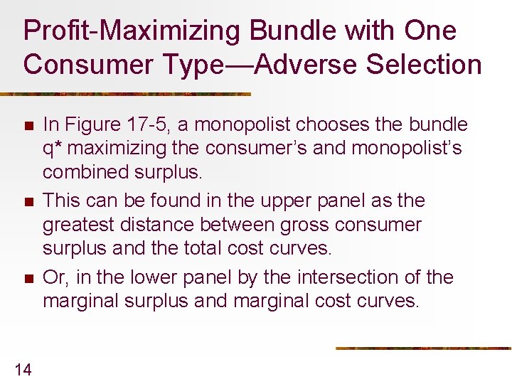
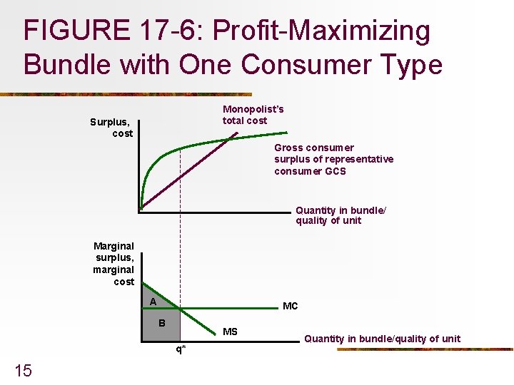
Profit-Maximizing Bundle with One Consumer Type—Adverse Selection n 14 In Figure 17 -5, a monopolist chooses the bundle q* maximizing the consumer’s and monopolist’s combined surplus. This can be found in the upper panel as the greatest distance between gross consumer surplus and the total cost curves. Or, in the lower panel by the intersection of the marginal surplus and marginal cost curves.

FIGURE 17 -6: Profit-Maximizing Bundle with One Consumer Type Monopolist’s total cost Surplus, cost Gross consumer surplus of representative consumer GCS Quantity in bundle/ quality of unit Marginal surplus, marginal cost A MC B MS q* 15 Quantity in bundle/quality of unit

FIGURE 17 -6: Comparing Gross and Ordinary Consumer Surplus Price ($/shirt) 15 7 A B E d 20 16 Quantity (shirts)

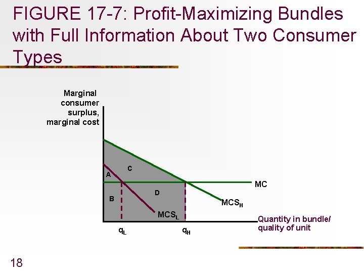
Two Consumer Types, Full Information n n 17 Facing a high-value and low-value consumer in Figure 17 -7, the monopolist chooses bundles given by the intersection between each type’s marginal consumer surplus and marginal cost. The high type receives a larger bundle q. H than the low type, q. L

FIGURE 17 -7: Profit-Maximizing Bundles with Full Information About Two Consumer Types Marginal consumer surplus, marginal cost C A MC D B MCSH MCSL q. L 18 q. H Quantity in bundle/ quality of unit

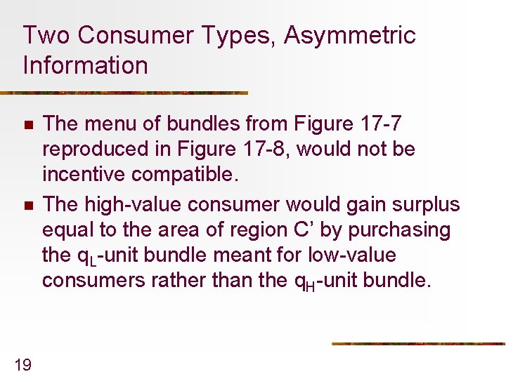
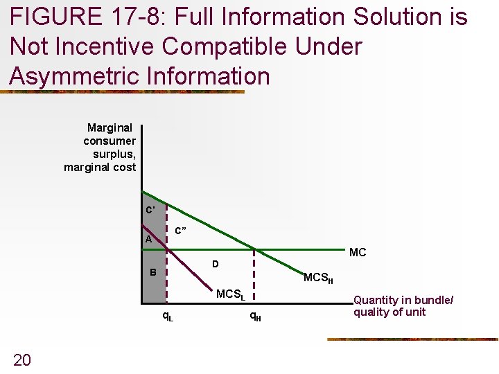
Two Consumer Types, Asymmetric Information n n 19 The menu of bundles from Figure 17 -7 reproduced in Figure 17 -8, would not be incentive compatible. The high-value consumer would gain surplus equal to the area of region C’ by purchasing the q. L-unit bundle meant for low-value consumers rather than the q. H-unit bundle.

FIGURE 17 -8: Full Information Solution is Not Incentive Compatible Under Asymmetric Information Marginal consumer surplus, marginal cost C’ C” A MC D B MCSH MCSL q. L 20 q. H Quantity in bundle/ quality of unit

Example: Insurance Industry n n 21 Insurance for car theft with some areas of high probability that a car will be stolen and some other areas thefts are quite rare. Suppose the insurance company offer the insurance based on the average theft rate. Only people lives in the high-risk areas will buy the insurance—adverse selection. Market outcomes are typically less efficient in the presence of the adverse-selection problem.

Signaling n n 22 The player with private information can take the first action and thereby signal something about his or her type. The first player makes a move called a signal since it is observed by the second player. Based on the information provided by the signal, the second player updates his or her beliefs about the first player’s type. Then the second player chooses his or her move and the game ends.

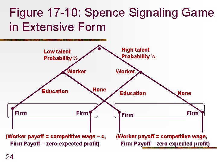
Spence Education Model n n 23 Spence’s education model, named after Michael Spence, who received the Nobel Prize in economics for developing it. The game tree for the Spence signaling game is shown in Figure 17 -10. Nature moves first, choosing the worker’s skill, low or high, with probability ½ each. The worker observes his or her skill and then makes the decision to get an education or not.

Figure 17 -10: Spence Signaling Game in Extensive Form . Low talent Probability ½ . . Firm Worker Education Worker None . Education . . Firm (Worker payoff = competitive wage – c, Firm Payoff – zero expected profit) 24 High talent Probability ½ Firm None Firm . (Worker payoff = competitive wage, Firm Payoff – zero expected profit)

Equilibrium of Signaling Games Signaling games often have multiple equilibria, and that is true in this game. n Separation equilibrium → Each type chooses a different action in a signaling game. n Pooling equilibrium → All types choose the same action in a signaling game. n 25