Chapter 3 Individual Demand Curves 2004 Thomson LearningSouthWestern

Chapter 3 Individual Demand Curves © 2004 Thomson Learning/South-Western

Individual Demand Curves l l l 2 This chapter studies how people change their choices when conditions such as income or changes in the prices of goods affect the amount that people choose to consume. This chapter then compares the new choices with those that were made before conditions changed The main result of this approach is to construct an individual’s demand curve

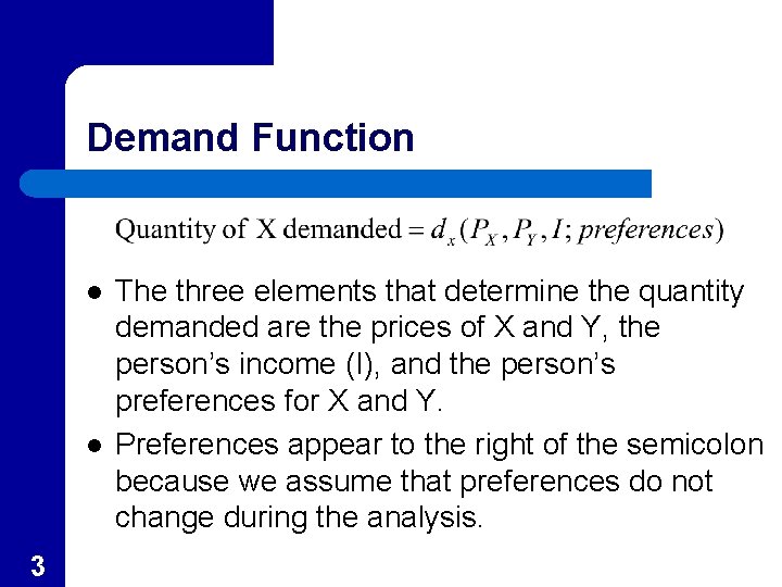
Demand Function l l 3 The three elements that determine the quantity demanded are the prices of X and Y, the person’s income (I), and the person’s preferences for X and Y. Preferences appear to the right of the semicolon because we assume that preferences do not change during the analysis.

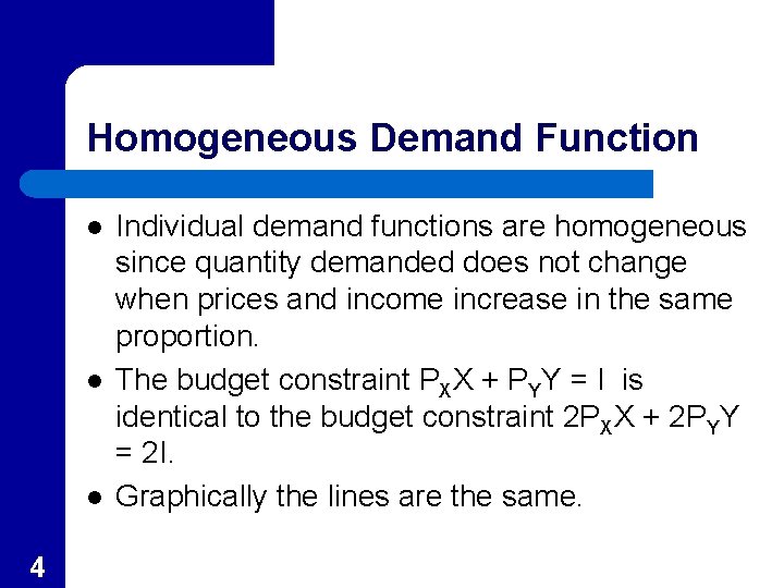
Homogeneous Demand Function l l l 4 Individual demand functions are homogeneous since quantity demanded does not change when prices and income increase in the same proportion. The budget constraint PXX + PYY = I is identical to the budget constraint 2 PXX + 2 PYY = 2 I. Graphically the lines are the same.

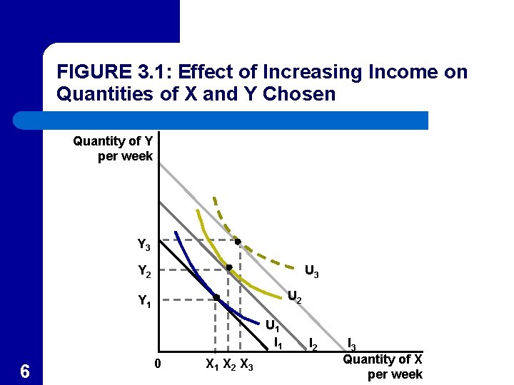
Changes in Income l l l 5 When a person’s income increase, while prices remain the same, the quantity purchased of each good might increase. This situation is shown in Figure 3. 1 where the increase in income is shown as the budget line shifts out from I 1 to I 2 to I 3. The slope of the budget lines are the same since the prices have not changed.

FIGURE 3. 1: Effect of Increasing Income on Quantities of X and Y Chosen Quantity of Y per week Y 3 Y 2 U 3 U 2 Y 1 U 1 I 1 6 0 X 1 X 2 X 3 I 2 I 3 Quantity of X per week

Normal Goods l l l 7 A normal good is one that is bought in greater quantities as income increases. If the quantity increases more rapidly than income the good is called a luxury good as with good Y in Figure 3. 1. If the quantity increases less rapidly than income the good is called a necessity good as with good X in Figure 3. 1.

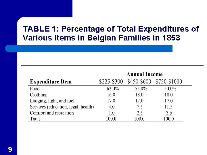
APPLICATION 3. 1: Engel’s Law l l l 8 One important generalization about consumer behavior is that the fraction of income spent on food tends to decline as income increases. This finding was discovered by Prussian economists Ernst Engel (1821 -1896). Table 1 show Engel’s data with Table 2 showing recent data for U. S. consumers.

TABLE 1: Percentage of Total Expenditures of Various Items in Belgian Families in 1853 9

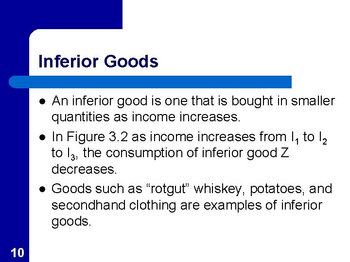
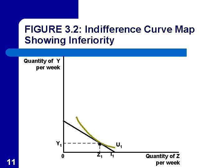
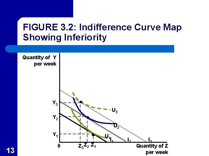
Inferior Goods l l l 10 An inferior good is one that is bought in smaller quantities as income increases. In Figure 3. 2 as income increases from I 1 to I 2 to I 3, the consumption of inferior good Z decreases. Goods such as “rotgut” whiskey, potatoes, and secondhand clothing are examples of inferior goods.

FIGURE 3. 2: Indifference Curve Map Showing Inferiority Quantity of Y per week Y 1 11 0 U 1 Z 1 I 1 Quantity of Z per week

FIGURE 3. 2: Indifference Curve Map Showing Inferiority Quantity of Y per week Y 2 U 2 Y 1 12 0 Z 2 Z 1 U 1 I 2 Quantity of Z per week

FIGURE 3. 2: Indifference Curve Map Showing Inferiority Quantity of Y per week Y 3 U 3 Y 2 U 2 Y 1 13 0 Z 3 Z 2 Z 1 U 1 I 2 I 3 Quantity of Z per week

Changes in a Good’s Price l l l 14 A change in the price of one good causes both the slope and an intercept of the budget line to change. The change also involves moving to a new utility-maximizing choice on another indifference curve with a different MRS. The quantity demanded of the good whose price has changed changes.

Substitution Effect l l l 15 The part of the change in quantity demanded that is caused by substitution of one good for another is called the substitution effect. This results in a movement along an indifference curve. Consumption has to be changed to equate MRS to the new price ratio of the two goods.

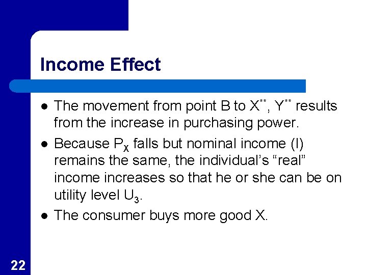
Income Effect l l 16 The part of the change in quantity demanded that is caused by a change in real income is called the income effect. The price change also changes “real” purchasing power and consumers will move to a new indifference curve that is consistent with this new purchasing power.

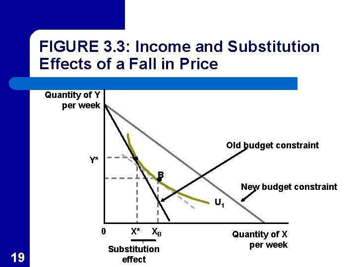
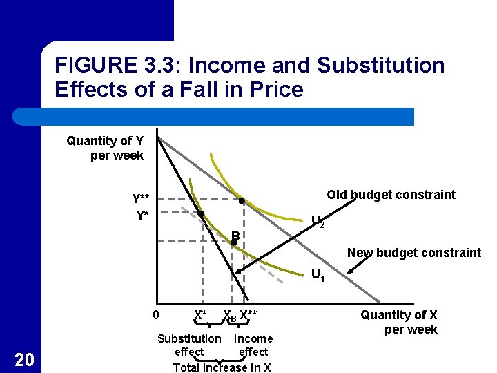
Substitution and Income Effects from a Fall in Price l l 17 As shown in Figure 3. 3, when the price of good X falls, the budget line rotates out from the unchanged Y axis so that the X intercept lies father out because the consumer can now buy more X with the lower price. The flatter slope means that the relative price of X to Y (PX/PY) has fallen.

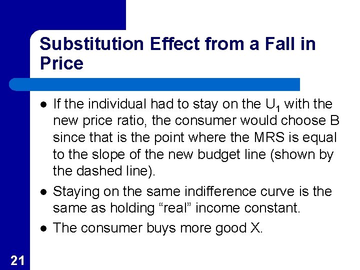
Substitution Effect from a Fall in Price l l l 18 The consumer was originally maximizing utility at X*, Y* in Figure 3. 3. After the fall in the price of good X, the new utility maximizing choice is X**, Y**. The substitution effect is the movement on the original indifference curve to point B.

FIGURE 3. 3: Income and Substitution Effects of a Fall in Price Quantity of Y per week Old budget constraint Y* B New budget constraint U 1 0 19 X* XB Substitution effect Quantity of X per week

FIGURE 3. 3: Income and Substitution Effects of a Fall in Price Quantity of Y per week Old budget constraint Y** Y* B U 2 New budget constraint U 1 0 20 X* XB X** Substitution Income effect Total increase in X Quantity of X per week

Substitution Effect from a Fall in Price l l l 21 If the individual had to stay on the U 1 with the new price ratio, the consumer would choose B since that is the point where the MRS is equal to the slope of the new budget line (shown by the dashed line). Staying on the same indifference curve is the same as holding “real” income constant. The consumer buys more good X.

Income Effect l l l 22 The movement from point B to X**, Y** results from the increase in purchasing power. Because PX falls but nominal income (I) remains the same, the individual’s “real” income increases so that he or she can be on utility level U 3. The consumer buys more good X.

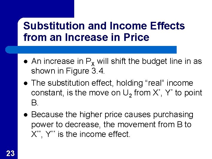
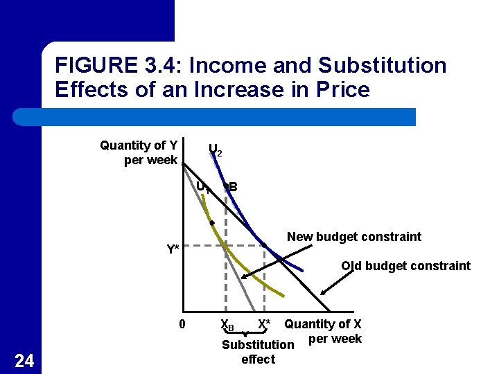
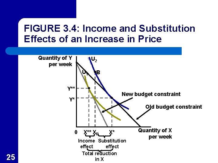
Substitution and Income Effects from an Increase in Price l l l 23 An increase in PX will shift the budget line in as shown in Figure 3. 4. The substitution effect, holding “real” income constant, is the move on U 2 from X*, Y* to point B. Because the higher price causes purchasing power to decrease, the movement from B to X**, Y** is the income effect.

FIGURE 3. 4: Income and Substitution Effects of an Increase in Price Quantity of Y per week U 2 U 1 B New budget constraint Y* Old budget constraint 0 24 XB X* Quantity of X Substitution per week effect

FIGURE 3. 4: Income and Substitution Effects of an Increase in Price Quantity of Y per week U 2 U 1 B Y** New budget constraint Y* Old budget constraint 0 25 X** XB X* Income Substitution effect Total reduction in X Quantity of X per week

Substitution and Income Effects for a Normal Good: Summary l l l 26 As shown in Figures 3. 3 and 3. 4, the substitution and income effects work in the same direction with a normal good. When the price falls, both the substitution and income effects result in more purchased. When the price increases, both the substitution and income effects result in less purchased.

Substitution and Income Effects for a Normal Good: Summary l l l 27 This provides the rational for drawing downward sloping demand curves. This also helps to determine the steepness of the demand curve. If either the substitution or income effects are large, the change in quantity demanded will be large with a given price change.

APPLICATION 3. 2: The Consumer Price Index and Its Biases l l 28 The Bureau of Labor Statistics monthly calculates the Consumer Price Index (CPI) which is a principal measure of inflation in the U. S. . To construct the CPI, a typical market basket of commodities purchased by consumers in the base year (currently 1982) is calculated.

An Algebraic Example l l l 29 Suppose the 1982 typical market basket contained X 82 of good X and Y 82 of good Y. The prices of these goods are and The cost of this bundle in the 1982 base year would be written as

An Algebraic Example l 30 To compute the cost of the same bundle of goods in, say 2002, requires that we compute the cost of the bundle using current prices

An Algebraic Example 31 l The CPI is defined as the ratio of the costs of these two market baskets l If the basket cost $100 in 1982 prices and $180 in 2002, the value of the CPI would be 1. 80 and with a measured 80 percent increase in prices over the 20 year period.

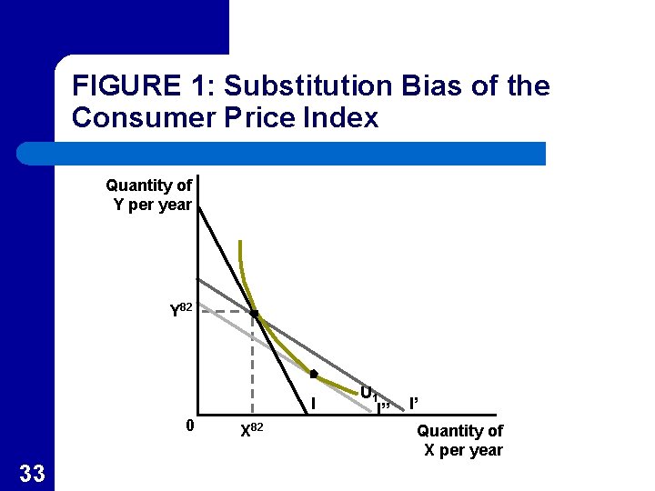
Substitution Bias in the CPI l l 32 The CPI does not take into account the real possibility that consumers would substitute among commodities because of changes in relative prices. In Figure 1, the typical individual is initially consuming X 82, Y 82 maximizing utility on U 1 with 1982 constraint I.

FIGURE 1: Substitution Bias of the Consumer Price Index Quantity of Y per year Y 82 I 0 33 X 82 U 1 I” I’ Quantity of X per year

Substitution Bias in the CPI l l l 34 Suppose the 2002 relative prices change so that PX/PY falls. The cost of the 1982 bundle in terms of 2002 prices is reflected in the constraint I’ which is flatter and goes though the 1982 bundle. The consumer would substitute X for Y and stay on U 1 on budget line I’’.

Substitution Bias in the CPI l l 35 Since I’’ is inside I’ (which is used to compute the CPI), the CPI tends to overstate the inflation rate. Unfortunately, adjusting the CPI to take such substitution into account is difficult because it would require that we know the utility function of the typical consumer.

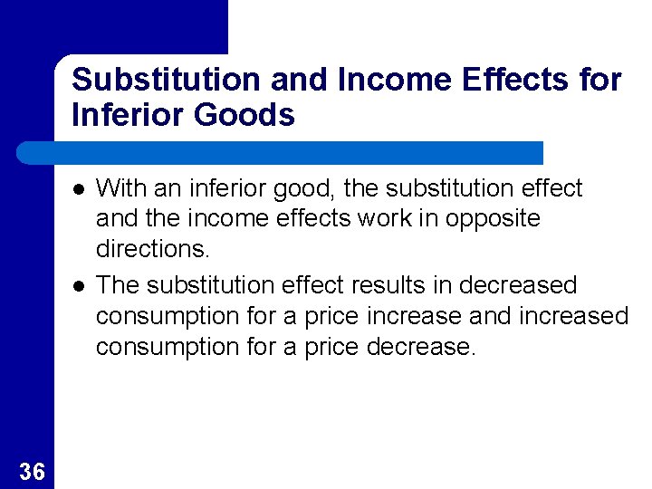
Substitution and Income Effects for Inferior Goods l l 36 With an inferior good, the substitution effect and the income effects work in opposite directions. The substitution effect results in decreased consumption for a price increase and increased consumption for a price decrease.

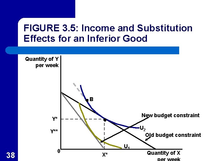
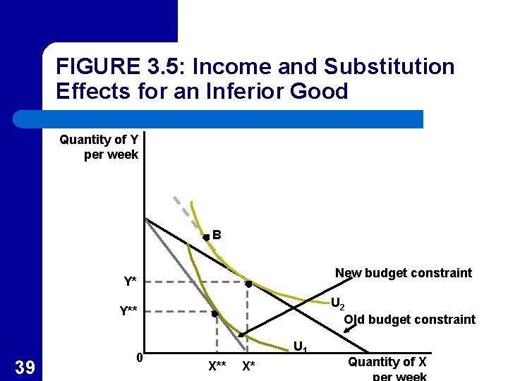
Substitution and Income Effects for Inferior Goods l l l 37 The income effect results in increased consumption for a price increase and decreased consumption for a price decrease. Figure 3. 5 shows the two effects for an increase in PX. The substitution effect, holding real income constant, is shown by the move from X*, Y* to point B both on U 2.

FIGURE 3. 5: Income and Substitution Effects for an Inferior Good Quantity of Y per week B New budget constraint Y* U 2 Old budget constraint Y** 38 0 U 1 X* Quantity of X

FIGURE 3. 5: Income and Substitution Effects for an Inferior Good Quantity of Y per week B New budget constraint Y* U 2 Old budget constraint Y** 39 0 U 1 X** X* Quantity of X

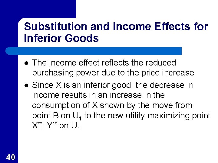
Substitution and Income Effects for Inferior Goods l l 40 The income effect reflects the reduced purchasing power due to the price increase. Since X is an inferior good, the decrease in income results in an increase in the consumption of X shown by the move from point B on U 1 to the new utility maximizing point X**, Y** on U 1.

Substitution and Income Effects for Inferior Goods l l l 41 Since X** is less than X* the price increase in X results in a decrease in the consumption of X. This occurs because the substitution effect, in this example, is bigger than the income effect. Thus, if the substitution effect dominates, the demand curve is negatively sloped.

Giffen’s Paradox l l 42 If the income effect of a price change is strong enough with an inferior good, it is possible for the quantity demanded to change in the same direction as the price change. Legend has it that this phenomenon was observed by English economist Robert Giffen.

Giffen’s Paradox l l l 43 When the price of potatoes rose in Ireland the consumption of potatoes also increased. Potatoes were not only an inferior good but constituted the source of a large portion of Irish people’s income. The situation I which an increase in a good’s price leads people to consume more of the good is called Giffen’s paradox.

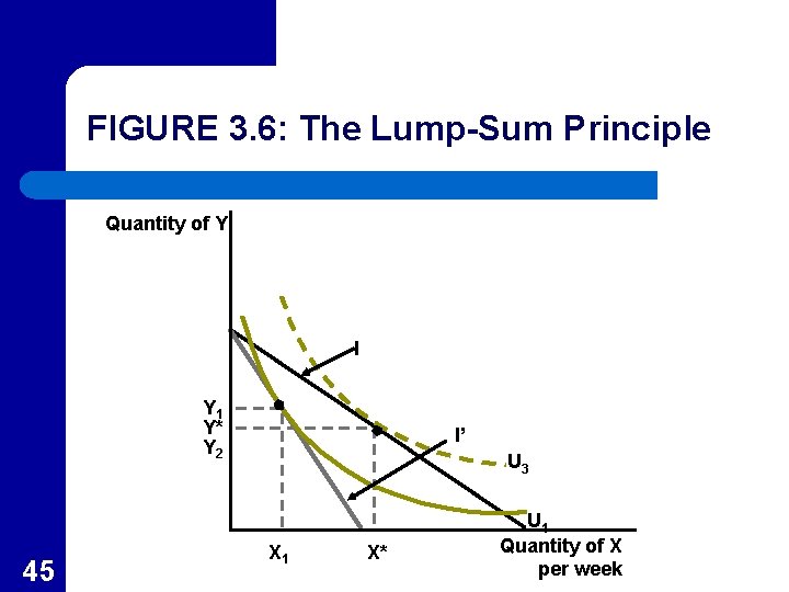
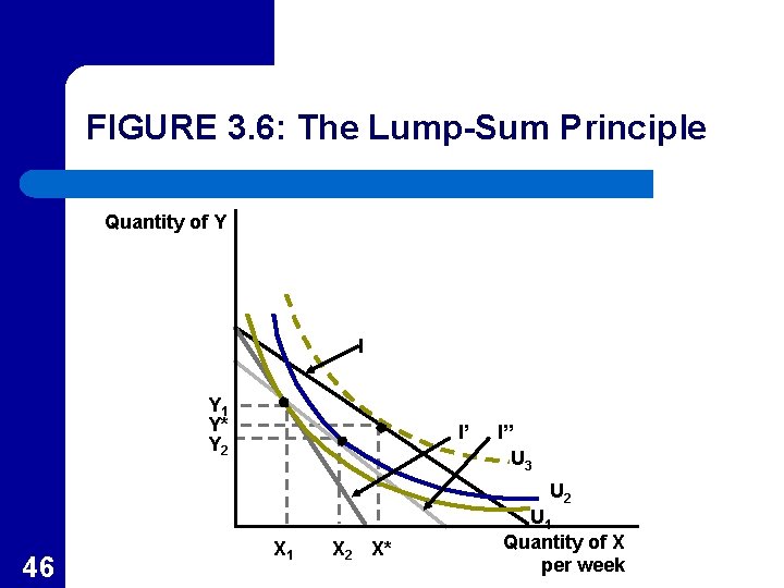
The Lump Sum Principle l l 44 The “lump-sum principle” hold that taxes that are imposed on general purchasing power will have a smaller welfare costs than will taxes imposed on a narrow selection of commodities. Consider Figure 3. 6 where the individual initially has I dollars to spend and chooses to consume X* and Y* yielding U 3 utility.

FIGURE 3. 6: The Lump-Sum Principle Quantity of Y I Y 1 Y* Y 2 45 I’ U 3 X 1 X* U 1 Quantity of X per week

FIGURE 3. 6: The Lump-Sum Principle Quantity of Y I Y 1 Y* Y 2 I’ I” U 3 U 2 46 X 1 X 2 X* U 1 Quantity of X per week

The Lump Sum Principle l l 47 The utility maximizing choice on I’’ is X 2, Y 2 yielding utility level U 2. The lump-sum general income tax generates the same amount of tax revenue but leaves the consumer on a higher utility level (U 2) than the utility level associated with the tax only on good X (U 1).

The Lump Sum Principle l The intuitive explanation of the lump-sum principle is that a single-commodity tax affects people in two ways: – – l 48 it reduces their purchasing power, it directs consumption away from the good being taxed. The lump-sum tax only has the first of these two effects.

Generalizations of the Lump-Sum Principle l l 49 The utility lass associated with the need to collect a certain amount of tax revenue will be minimized by taxing goods for which the substitution effect is small. Even though the tax will reduce purchasing power, it will minimize the impact of directing consumption away from the good being taxed.

APPLICATION 3. 3: Wouldn’t Cash Be a Better Way to Help Poor People? l l 50 The lump-sum principle suggests that the trends in expanding in-kind programs may be unfortunate These programs do not generate as much welfare for people as would the spending of the same funds in a cash program

FIGURE 1: The Superiority of an Income Grant Y period I’’ U 3 B I U 2 U 1 51 I’ X period

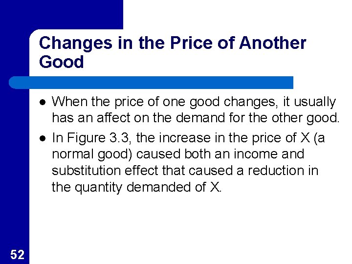
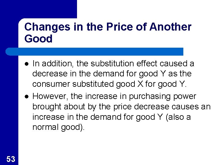
Changes in the Price of Another Good l l 52 When the price of one good changes, it usually has an affect on the demand for the other good. In Figure 3. 3, the increase in the price of X (a normal good) caused both an income and substitution effect that caused a reduction in the quantity demanded of X.

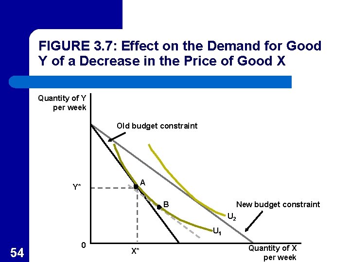
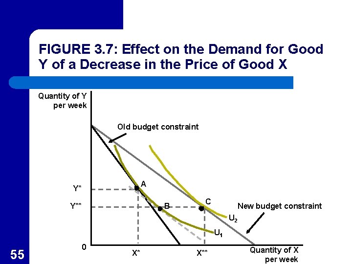
Changes in the Price of Another Good l l 53 In addition, the substitution effect caused a decrease in the demand for good Y as the consumer substituted good X for good Y. However, the increase in purchasing power brought about by the price decrease causes an increase in the demand for good Y (also a normal good).

FIGURE 3. 7: Effect on the Demand for Good Y of a Decrease in the Price of Good X Quantity of Y per week Old budget constraint A Y* B New budget constraint U 2 U 1 54 0 X* Quantity of X per week

FIGURE 3. 7: Effect on the Demand for Good Y of a Decrease in the Price of Good X Quantity of Y per week Old budget constraint A Y* Y** B C New budget constraint U 2 U 1 55 0 X* X** Quantity of X per week

Changes in the Price of Another Good l l 56 However, in this case, the income effect is much smaller than the substitution effect so that the consumer ends up consuming less of good Y at Y** after the decrease in the price of X. Thus, the effect of a change in the price of one good has an ambiguous effect on the demand for the other good.

Complements l l 57 Complements are goods that go together in the sense that people will increase their use of both goods simultaneously. Two goods are complements if an increase in the price of one causes a decrease in the demanded of the other or a decrease in the price of one good causes an increase in the demand for the other.

Substitutes l l l 58 Substitutes are goods that are used for essentially the same purpose. Two goods such that if the price of one increases, the demand for the other rises are substitutes. If the price of one good decreases and the demand for the other good decreases, they are also substitutes.

Construction of Individual Demand Curves l l 59 An individual demand curve is a graphic representation between the price of a good and the quantity of it demanded by a person holding all other factors (preferences, the prices of other goods, and income) constant. Demand curves limit the study to the relationship between the quantity demanded and changes in the own price of the good.

Construction of Individual Demand Curves l l l 60 In Panel a of Figure 3. 8 an individual’s indifference curve map is drawn using three different budget constraints in which the price of X decreases. The decreasing prices are P’X, P”X, and P’’’X respectively. The individual’s utility maximizing choices of X are X’, and X’’’ respectively.

FIGURE 3. 8: Construction of an Individual’s Demand Curve Quantity of Y per week Budget constraint for P’X Budget constraint for P’’’X U 3 U 2 U 1 0 X’ X” Quantity of X per week (a) Individual’s indifference curve map Price X’” P 9 X P 0 X PX 61 0 X’ X” X’” (b) Demand curve Quantity of X per week

FIGURE 3. 8: Construction of an Individual’s Demand Curve Quantity of Y per week Budget constraint for P’X Budget constraint for P’’’X U 3 U 2 U 1 0 X’ X” Quantity of X per week (a) Individual’s indifference curve map Price X’” P 9 X P 0 X PX 62 d 0 X’ X” X X’” (b) Demand curve Quantity of X per week

Construction of Individual Demand Curves l l 63 These three choices show that the quantity demanded of X increases as the price of X falls. Panel b shows how the three price and quantity choices can be used to construct the demand curve.

Shape of the Demand Curve l If a good, say X, has close substitutes, a increase in its price will cause a large decrease in the quantity demanded as the substitution effect will be large. – 64 The demand curve for a type of breakfast cereal will likely be relatively flat due to the strong substitution effect.

Shape of the Demand Curve l l 65 Food has no substitutes so it might be thought that no change in consumption would occur with a price increase. But food constitutes a large part of an individual’s budget so that price changes will cause relatively larger effects on the quantity demanded that might be thought due to the income effect.

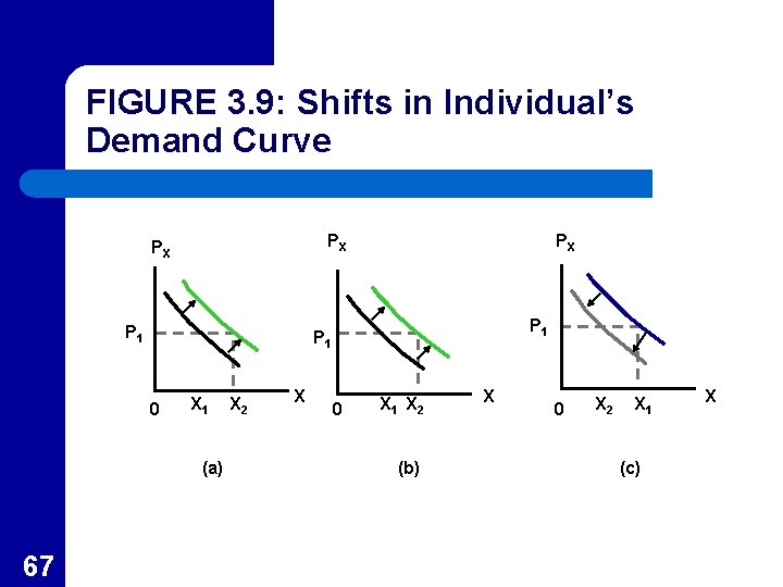
Shifts in an Individual’s Demand Curve l l l 66 When one of the variables that are held constant (price of another good, income or preferences) on a demand curve changes, the entire curve shifts. Figure 3. 9 shows the kinds of shifts that might take place. If X is a normal good and income increases, demand increases as shown in Panel a.

FIGURE 3. 9: Shifts in Individual’s Demand Curve PX PX P 1 P 1 0 X 1 (a) 67 PX X 2 X 0 X 1 X 2 (b) X 0 X 2 X 1 (c) X

Shifts in an Individual’s Demand Curve l l 68 If X and Y are substitutes and the price of Y increases, the demand for X increases as shown in Panel b. Alternatively, if X and Y are complements, the increase in the price of Y will cause a decrease in the demand for X as shown in Panel c.

Shifts in an Individual’s Demand Curve l l l 69 Changes in preferences can also shift demand curves. Panel b could represent an increased preference for cold drinks when a sudden hot spell occurs. Increased environmental consciousness during the 1980’s and 1990 s increased the demand for recycling and organic food.

APPLICATION 3. 5: Fads, Seasons, and Health Scares l Health scares can cause large decreases in the demand for products. – l 70 Examples include the long term decline in smoking and the decreased demand for Chinese food because of the concern for its fat content. Recent “scientific” studies have also affected demand such as the increase in the demand for tomatoes in 1998.

Be Careful in Using Terminology l l 71 A movement downward along a stationary demand curve in response to a fall in price is called an increase in quantity demanded while a rise in the price of the good results in a decrease in quantity demanded. A rightward shift in a demand curve is called an increase in demand while a leftward shift is a decrease in demand.

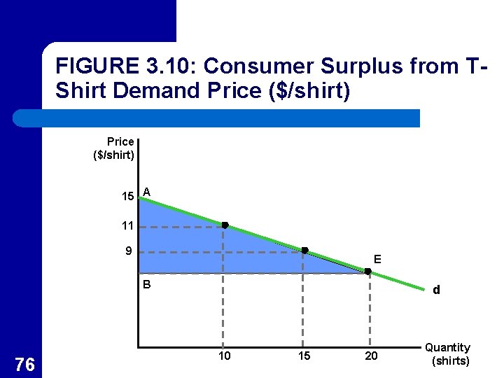
Consumer Surplus l l l 72 The extra value individuals receive from consuming a good over what they pay for it is called consumer surplus. Consumer surplus is also what people would be willing to pay for the right to consume a good at its current price. This concept is used to study the welfare effects of price changes.

Consumer Surplus l l l 73 Because a good is usually sold at a single market price, people choose to buy additional units of the good up to the point at which their marginal valuation is equal to the price. In Figure 3. 10, if T-shirts sell for $7, the individual will buy twenty shirts because the twentieth T-shirt is worth precisely $7. They will not buy the twenty-first T-shirt because it is worth less than $7.

Consumer Surplus l l 74 Because the individual would be willing to pay more than $7 for the tenth or fifteenth T-shirt, it is clear that they get a “surplus” on those shirts because the individual is actually paying less than the maximal amount that they would be willing to pay. Consumer surplus is the difference between the maximal amounts a person would pay for a good and what he or she actually pays.

Consumer Surplus In graphical terms, consumer surplus is given by the area below the demand curve and above the market price. l In Figure 3. 10, total consumer surplus is given by area AEB ($80). l 75

FIGURE 3. 10: Consumer Surplus from TShirt Demand Price ($/shirt) 15 A 11 9 E B 76 d 10 15 20 Quantity (shirts)

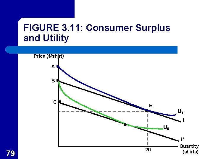
Consumer Surplus and Utility l l l 77 Figure 3. 11 illustrates the connection between consumer surplus and utility Initially, the person is at E with utility U 1. He or she would need to be compensated by amount AB in other goods to get U 1 if T -shirts were not available.

Consumer Surplus and Utility l l 78 In Figure 3. 11, the individual would be willing to pay BC for the right to consume T -shirts rather than spending I only on other goods. Both distance AB and BC approximate the consumer surplus area in Figure 3. 10.

FIGURE 3. 11: Consumer Surplus and Utility Price ($/shirt) A B C E U 1 I U 0 I’ 79 20 Quantity (shirts)

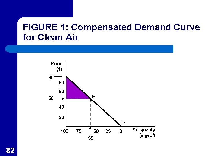
APPLICATION 3. 6: Valuing Clean Air l l 80 By looking at the ceteris paribus relationship between air pollution levels in various locations and the prices of houses in these locations, it is possible to infer the amount that people will pay to avoid dirty air. This information allows the computation of a compensated demand curve for clean air.

APPLICATION 3. 6: Valuing Clean Air l l 81 In Figure 1, the vertical axis shows the price home buyers are willing to pay to avoid air pollution and the horizontal axis shows the quantity of clean air purchased. The national average is reflected at point E as home buyers pay $50 and consume an average of 55 micrograms of suspended particulates per cubic meter.

FIGURE 1: Compensated Demand Curve for Clean Air Price ($) 85 80 60 E 50 40 20 D 100 75 50 55 82 25 0 Air quality (mg/m 3)

APPLICATION 3. 6: Valuing Clean Air l l l 83 Consumers are paying $2, 250 ($50 times 45 micrograms) extra to avoid dirty air. At E 0 consumers also receive a consumer surplus equal to the shaded area in Figure 1. This consumer surplus of 788 per household can be multiplied by the total number of households to estimate total consumer surplus from clean air.