Molecular systematics QTL Quantitative trait locus analysis use

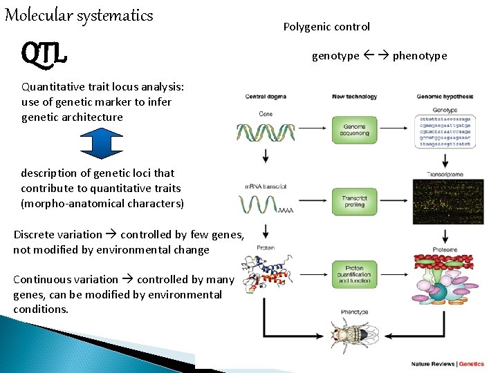
Molecular systematics QTL Quantitative trait locus analysis: use of genetic marker to infer genetic architecture description of genetic loci that contribute to quantitative traits (morpho-anatomical characters) Discrete variation controlled by few genes, not modified by environmental change Continuous variation controlled by many genes, can be modified by environmental conditions. Polygenic control genotype phenotype

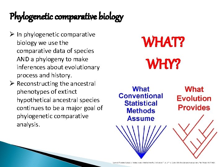
Phylogenetic comparative biology Ø In phylogenetic comparative biology we use the comparative data of species AND a phylogeny to make inferences about evolutionary process and history. Ø Reconstructing the ancestral phenotypes of extinct hypothetical ancestral species continues to be a major goal of phylogenetic comparative analysis. WHAT? WHY?

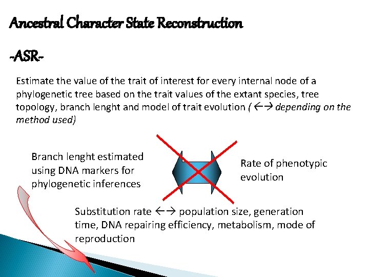
Ancestral Character State Reconstruction -ASREstimate the value of the trait of interest for every internal node of a phylogenetic tree based on the trait values of the extant species, tree topology, branch lenght and model of trait evolution ( depending on the method used) Branch lenght estimated using DNA markers for phylogenetic inferences Rate of phenotypic evolution Substitution rate population size, generation time, DNA repairing efficiency, metabolism, mode of reproduction

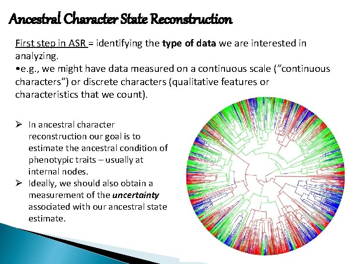
Ancestral Character State Reconstruction First step in ASR = identifying the type of data we are interested in analyzing. • e. g. , we might have data measured on a continuous scale (“continuous characters”) or discrete characters (qualitative features or characteristics that we count). Ø In ancestral character reconstruction our goal is to estimate the ancestral condition of phenotypic traits – usually at internal nodes. Ø Ideally, we should also obtain a measurement of the uncertainty associated with our ancestral state estimate.

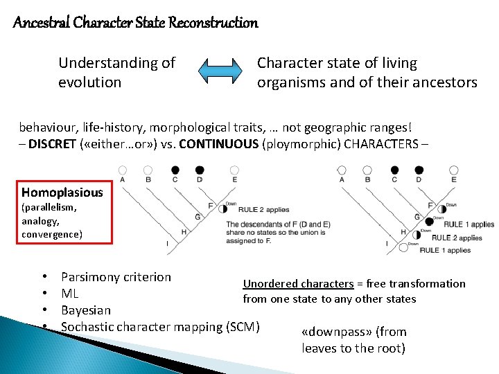
Ancestral Character State Reconstruction Understanding of evolution Character state of living organisms and of their ancestors behaviour, life-history, morphological traits, … not geographic ranges! – DISCRET ( «either…or» ) vs. CONTINUOUS (ploymorphic) CHARACTERS – Homoplasious (parallelism, analogy, convergence) • • Parsimony criterion Unordered characters = free transformation ML from one state to any other states Bayesian Sochastic character mapping (SCM) «downpass» (from leaves to the root)

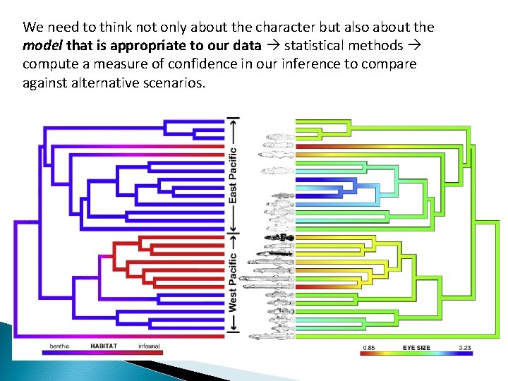
We need to think not only about the character but also about the model that is appropriate to our data statistical methods compute a measure of confidence in our inference to compare against alternative scenarios.

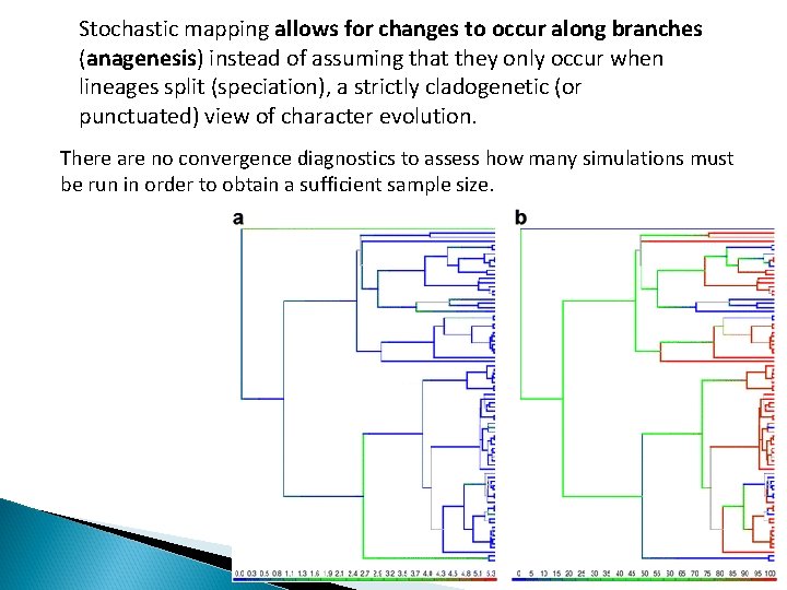
Stochastic mapping allows for changes to occur along branches (anagenesis) instead of assuming that they only occur when lineages split (speciation), a strictly cladogenetic (or punctuated) view of character evolution. There are no convergence diagnostics to assess how many simulations must be run in order to obtain a sufficient sample size.

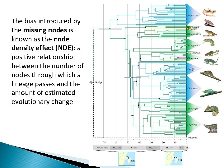
The bias introduced by the missing nodes is known as the node density effect (NDE): a positive relationship between the number of nodes through which a lineage passes and the amount of estimated evolutionary change.

Ancestral Character State Reconstruction Joint vs. marginal reconstruction Ø Joint ASR is finding the set of character states at all nodes throughout the tree that (jointly) maximize the likelihood of the data. Computationally complex but already optimized! Ø Marginal ASR is finding the state at the current node that maximizes the likelihood integrating over all other states at all nodes, in proportion to their probability;

Ancestral Character State Reconstruction ØAt each node the set of empirical Bayesian posterior probabilities that each node is in each state is computed. ØIt works upwards from the descendants of a tree to progressively assign the most likely character state to each ancestor taking into consideration only its immediate descendants Øalgorithm that makes the locally optimal choice at each stage of the optimization problem. ØWhile it can be highly efficient, it is not guaranteed to attain a globally optimal solution to the problem.

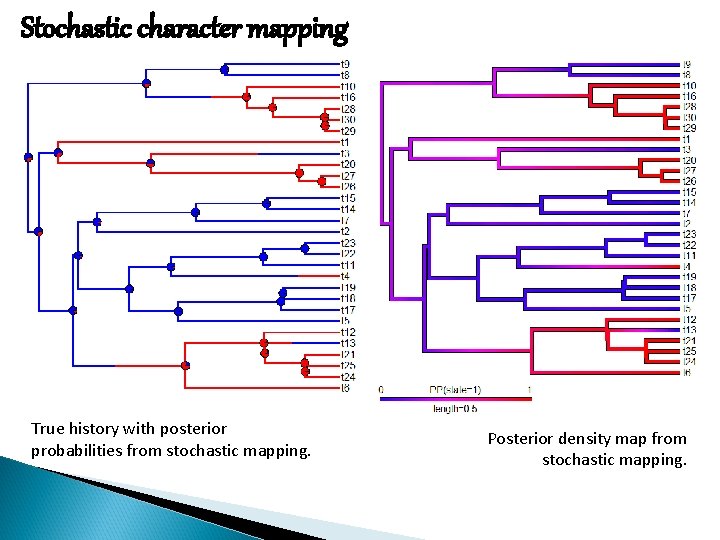
Joint ASR: Ø is finding the set of states at all internal nodes that maximize the likelihood. Ø This is not (necessarily) equivalent to picking the state at each node with the highest probability. Ø We can find the single character history with the highest likelihood – but this is just one sample from the distribution. It happens to be the most likely, but it doesn’t contain any information about uncertainty. Ø One option is to sample node states and character histories from their joint (empirical or heirarchical) Bayesian posterior distribution stochastic character mapping.

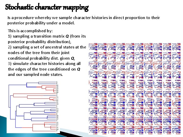
Stochastic character mapping Is a procedure whereby we sample character histories in direct proportion to their posterior probability under a model. This is accomplished by: 1) sampling a transition matrix Q (from its posterior probability distribution), 2) sampling a set of ancestral states at the nodes of the tree from their joint conditional probability dist. given Q, 3) simulate character histories along all the edges of the tree conditioned on Q and our sampled node states.

Stochastic character mapping True history with posterior probabilities from stochastic mapping. Posterior density map from stochastic mapping.

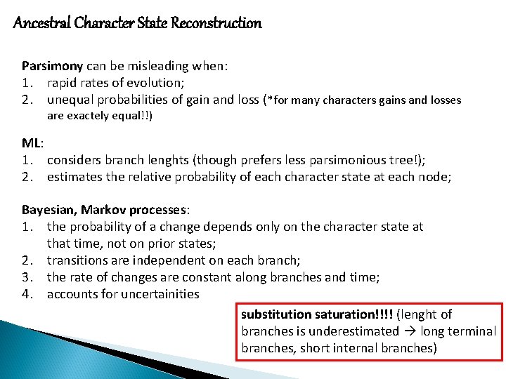
Ancestral Character State Reconstruction Parsimony can be misleading when: 1. rapid rates of evolution; 2. unequal probabilities of gain and loss (*for many characters gains and losses are exactely equal!!) ML: 1. considers branch lenghts (though prefers less parsimonious tree!); 2. estimates the relative probability of each character state at each node; Bayesian, Markov processes: 1. the probability of a change depends only on the character state at that time, not on prior states; 2. transitions are independent on each branch; 3. the rate of changes are constant along branches and time; 4. accounts for uncertainities substitution saturation!!!! (lenght of branches is underestimated long terminal branches, short internal branches)

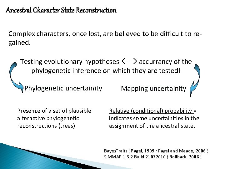
Ancestral Character State Reconstruction Complex characters, once lost, are believed to be difficult to regained. Testing evolutionary hypotheses accurrancy of the phylogenetic inference on which they are tested! Phylogenetic uncertainity Presence of a set of plausible alternative phylogenetic reconstructions (trees) Mapping uncertainity Relative (conditional) probability = indicates some uncertainities in the assignment of the ancestral state. Bayes. Traits ( Pagel, 1999 ; Pagel and Meade, 2006 ) SIMMAP 1. 5. 2 Build 21072010 ( Bollback, 2006 )

Ancestral Character State Reconstruction Ø The mean difference between reconstructions is smaller when more taxa are present in the analysis. Ø For MP methods, larger taxon sampling does not necessarily lead to a more accurate reconstruction (Li et al. 2008). Ø Taxon sampling matters for ML and Bayesian methods for accurate ancestral character state reconstruction (Heath et al. 2008). If the rate of molecular evolution explains part of the phenotypic variation between species, inferring ancestral character states on time-calibrated trees (chronogram) could have deceiving results not appropriate representation of trait evolution of the species.

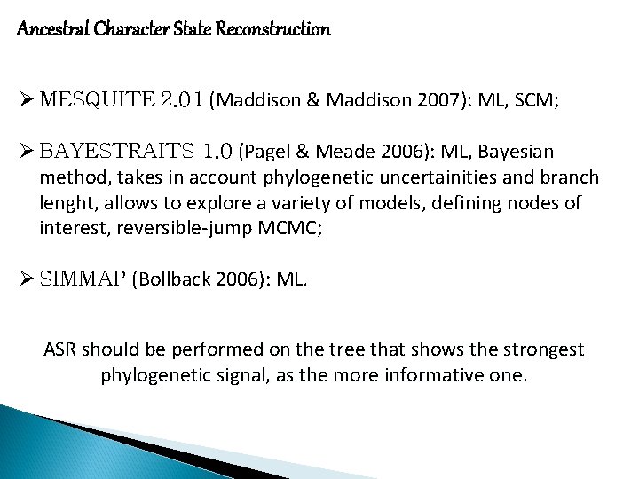
Ancestral Character State Reconstruction Ø MESQUITE 2. 01 (Maddison & Maddison 2007): ML, SCM; Ø BAYESTRAITS 1. 0 (Pagel & Meade 2006): ML, Bayesian method, takes in account phylogenetic uncertainities and branch lenght, allows to explore a variety of models, defining nodes of interest, reversible-jump MCMC; Ø SIMMAP (Bollback 2006): ML. ASR should be performed on the tree that shows the strongest phylogenetic signal, as the more informative one.

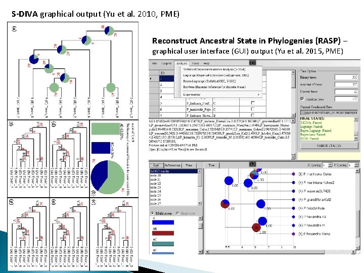
S-DIVA graphical output (Yu et al. 2010, PME) Reconstruct Ancestral State in Phylogenies (RASP) – graphical user interface (GUI) output (Yu et al. 2015, PME)

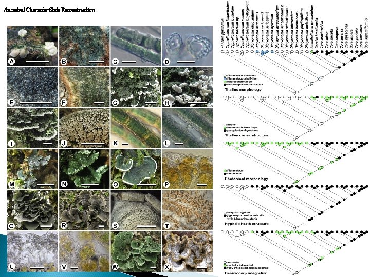
Ancestral Character State Reconstruction

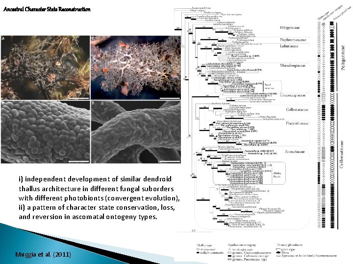
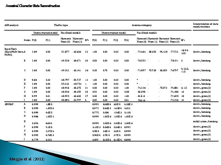
Ancestral Character State Reconstruction i) independent development of similar dendroid thallus architecture in different fungal suborders with different photobionts (convergent evolution), ii) a pattern of character state conservation, loss, and reversion in ascomatal ontogeny types. Muggia et al. (2011)

Ancestral Character State Reconstruction ASR analysis Thallus type Unconstrained model Nodes P(0) Interpretation of state reconstruction Ascoma ontogeny Fossilized models Unconstrained model Fossilized models P(1) Harmonic BFs Mean (0) Mean (1) P(0) P(1) P(2) P(3) Harmonic BFs Mean (0) Mean (1) Mean (2) Mean (3) Bayes. Traits (Bayes. Multi State, A MCMC) 1. 00 0. 00 -51. 877 -62. 636 22 1. 00 0. 00 -72. 464 -80. 350 -94. 128 -77. 722 16; 43; 10. 5 dorsiv. , hemiang. B 1. 00 0. 00 -49. 510 -64. 471 30 0. 50 0. 00 0. 50 -76. 552 - - -78. 191 3 dorsiv. , hemiang. C 1. 00 0. 00 -49. 241 -62. 141 26 0. 25 0. 75 0. 00 -71. 097 -75. 735 -82. 359 -76. 797 9; 22. 5; 11. 5 dorsiv. , hemiang. D 0. 66 0. 33 -48. 797 -54. 727 12 1. 00 0. 00 * - - dorsiv. , hemiang. E 1. 00 0. 00 -49. 216 -48. 754 1 1. 00 0. 00 * - - dorsiv. , hemiang. F 1. 00 0. 00 -48. 916 -64. 375 31 0. 00 1. 00 -74. 116 - -75. 473 -74. 881 3; 1. 5 dorsiv. , gymn. (3) G 1. 00 0. 00 -48. 916 -64. 259 30 0. 92 0. 00 0. 08 -82. 398 - - -74. 186 16 dorsiv. , gymn. (3) H 0. 99 0. 01 -48. 925 -62. 630 27 0. 00 1. 00 -81. 513 - - -72. 620 18 dorsiv. , gymn. (3) I 1. 00 0. 00 -50. 893 -52. 797 4 0. 49 0. 00 0. 51 -78. 216 - - -73. 216 10 dorsiv. , gymn. (3) A 0. 999 1. 8 E-5 0. 995 8. 38 E-4 6. 5 E-5 4. 28 E-3 B 0. 999 1. 39 E-4 0. 972 5. 46 E-3 1. 43 E-4 0. 022 dorsiv. , hemiang. C 0. 999 4. 4 E-5 0. 775 0. 084 1. 96 E-3 0. 138 dorsiv. , hemiang. D 0. 986 1. 35 E-2 0. 999 1. 00 E-6 dorsiv. , hemiang. 0. 396 0. 603 0. 999 2. 00 E-6 F 0. 999 9. 1 E-5 3. 10 E-3 5. 06 E-4 3. 56 E-3 0. 992 dorsiv. , gymn. (3) G 0. 999 2. 27 E-4 4. 9 E-5 2. 4 E-5 3. 4 E-5 0. 999 dorsiv. , gymn. (3) H 0. 995 4. 76 E-3 5. 94 E-4 3. 7 E-5 0. 999 dorsiv. , gymn. (3) I 0. 779 0. 220 0. 099 8. 15 E-4 0. 898 dorsiv. , gymn. (3) SIMMAP E Muggia et al. (2011) 8. 15 E-4 dorsiv. , hemiang. radial. symm. , hemiang.

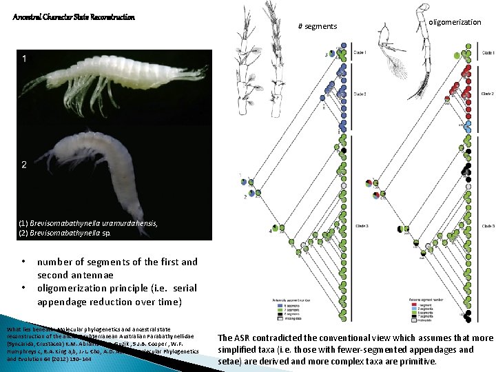
Ancestral Character State Reconstruction # segments oligomerization (1) Brevisomabathynella uramurdahensis, (2) Brevisomabathynella sp. • • number of segments of the first and second antennae oligomerization principle (i. e. serial appendage reduction over time) What lies beneath: Molecular phylogenetics and ancestral state reconstruction of the ancient subterranean Australian Parabathynellidae (Syncarida, Crustacea) K. M. Abrams M. T. Guzik , S. J. B. Cooper , W. F. Humphreys c, R. A. King a, b, J. -L. Cho, A. D. Austin, Molecular Phylogenetics and Evolution 64 (2012) 130– 144 The ASR contradicted the conventional view which assumes that more simplified taxa (i. e. those with fewer-segmented appendages and setae) are derived and more complex taxa are primitive.

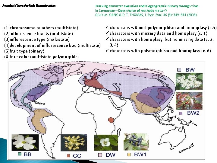
Ancestral Character State Reconstruction Tracking character evolution and biogeographic history through time in Cornaceae—Does choice of methods matter? Qiu-Yun XIANG & D. T. THOMAS, J. Syst. Evol. 46 (3): 349– 374 (2008) (1)chromosome numbers (multistate) (2)Inflorescence bracts (multistate) (3)inflorescence type (multistate) (4)development of inflorescence bud (multistate) (5)fruit type (binary) (6)fruit color (multistate polymorphic) ü characters without polymorphism and homoplasy (c. 5) ü characters with missing data and homoplasy (c. 1) ü characters with homoplasy, but no missing data (c. 2, 3, 4) ü characters with polymorphism and homoplasy (c. 6)

Ancestral Character State Reconstruction Tracking character evolution and biogeographic history through time in Cornaceae—Does choice of methods matter? Qiu-Yun XIANG & D. T. THOMAS, J. Syst. Evol. 46 (3): 349– 374 (2008) • 3 methods: - BAYESTRAITS, SIMMAP (estimates the instantaneous rates of character change using likelihood and accommodates phylogenetic uncertainty by evaluating the ancestral character state on trees sampled from the posterior distribution); - Stochastic character mapping (SCM), MESQUITE 2. 01 - parsimony-based dispersal-vicariance analysis = DIVA, used for ancestral distributions (finds the best biogeographic pathways given the tree topology and distributions of taxa by minimizing dispersal and extinction events) • chronograms and phylograms Reconstruction of the ancestral state with missing data is sensitive to branch length (or time available for evolution). The impact of method choice depends on the nature of characters. Characters with no homoplasy, no polymorphism, and no missing data reconstruction of the ancestral state was consistent among all methods compared and between topology-based and chronogram-based analyses choice of methods does not affect the inference of evolutionary trend (analysis using a chronogram better provides temporal information on character state transitions).

Molecular dating – tree calibration The genetic divergence between sequences is converted into absolute time. Two source of independent age-related information can be exploited: 1. To assign date to the MRCAs (internal nodes) 2. To use the information about the age of the sequenced samples by assigning dates to the tips (terminal nodes) tip-dating = (TED= total evidence dating) dated sequences contain sufficient information for populations to be characterized as “misurable evolving” (MEP).

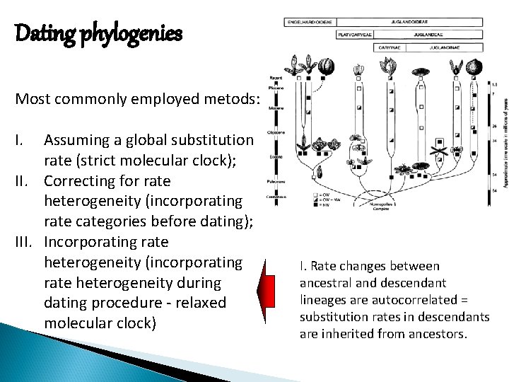
Dating phylogenies Most commonly employed metods: I. Assuming a global substitution rate (strict molecular clock); II. Correcting for rate heterogeneity (incorporating rate categories before dating); III. Incorporating rate heterogeneity (incorporating rate heterogeneity during dating procedure - relaxed molecular clock) I. Rate changes between ancestral and descendant lineages are autocorrelated = substitution rates in descendants are inherited from ancestors.

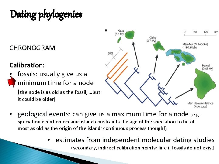
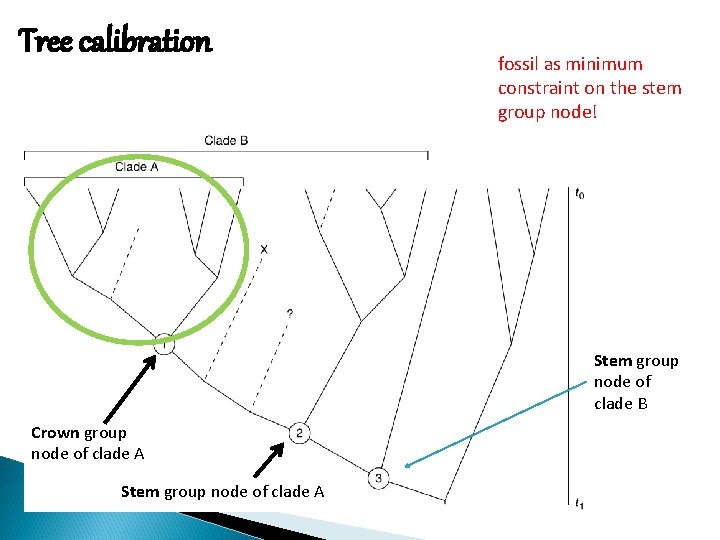
Dating phylogenies CHRONOGRAM Calibration: • fossils: fossils usually give us a minimum time for a node (the node is as old as the fossil, …but it could be older) • geological events: events can give us a maximum time for a node (e. g. speciation event on oceanic island constraints the age of the speciation to be at most as old as the origin of the island; continuous process though!) • estimates from independent molecular dating studies (secondary, indirect calibration points; fine if fossils do not exist)

Dating phylogenies Sources of error: 1. including phylogenetic uncertainty 2. substitution noise and saturation 3. rate heterogeneity (among lineages, over time and between DNA regions) 4. incomplete taxon sampling 5. incorrect branch length optimization 6. erroneous fossil age estimates (age of fossil as minimum constraint in calibration procedures = that clade cannot be younger than the fossil!) better to use multiple fossils! 7. incompleteness of the fossil record 8. placement of fossils on phylogenetic trees

Tree calibration fossil as minimum constraint on the stem group node! Stem group node of clade B Crown group node of clade A Stem group node of clade A

Tree calibration BEAST, Bayesian evolutionary analysis by sampling trees (Drummond and Rambaut, 2007) applies MCMC; simultaneously it i) searches the tree space to find the topologies plausible for your data, ii) estimate the rate of evolution and divergence time of each branch. v. BEAST-estimated divergence time = summary of estimations based on all the optimal Bayesian trees found in the analysis; it takes phylogenetic uncertainty into account, no rate autocorrelation (model and rates of evolution, topology )!!!

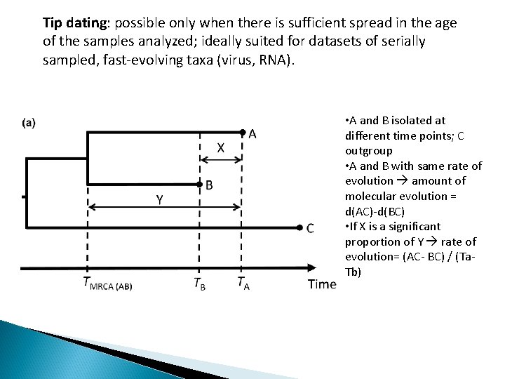
Tip dating: possible only when there is sufficient spread in the age of the samples analyzed; ideally suited for datasets of serially sampled, fast-evolving taxa (virus, RNA). • A and B isolated at different time points; C outgroup • A and B with same rate of evolution amount of molecular evolution = d(AC)-d(BC) • If X is a significant proportion of Y rate of evolution= (AC- BC) / (Ta. Tb)

tip-dating = dated sequences contain sufficient information for populations to be characterized as “misurable evolving” (MEP). MEP = population exibiting detectable amounts of de novo nucleotide changes among DNA sequences sampled at different time points. EPS = effective population size: the number of idealized individual that contribute the offspring to the descendent generation, it is almost always smaller than the census population size.

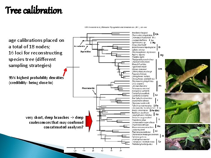
Tree calibration age calibrations placed on a total of 18 nodes; 16 loci for reconstructing species tree (different sampling strategies) 95% highest probability densities (credibility- being close to) very short, deep branches deep coalescences that may confound concatenated analyses?

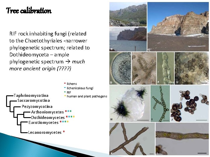
Tree calibration RIF rock inhabiting fungi (related to the Chaetothyriales -narrower phylogenetic spectrum; related to Dothideomyceta – ample phylogenetic spectrum much more ancient origin (? ? ) * lichens * lichenicolous fungi * RIF * human and plant pathogens Taphrinomycotina Saccaromycotina Pezyzomycotina Arthoniomycetes *** Dothideomycetes **** Eurotiomycetes **** Lecanoromycetes *

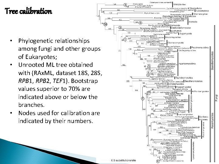
Tree calibration • Phylogenetic relationships among fungi and other groups of Eukaryotes; • Unrooted ML tree obtained with (RAx. ML, dataset 18 S, 28 S, RPB 1, RPB 2, TEF 1). Bootstrap values superior to 70% are indicated above or below the branches. • Nodes used for calibration are indicated by their numbers.

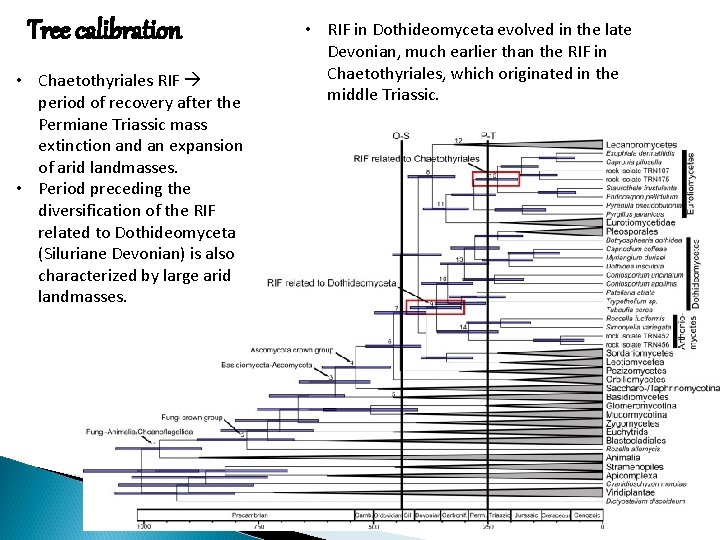
Tree calibration • Chaetothyriales RIF period of recovery after the Permiane Triassic mass extinction and an expansion of arid landmasses. • Period preceding the diversification of the RIF related to Dothideomyceta (Siluriane Devonian) is also characterized by large arid landmasses. • RIF in Dothideomyceta evolved in the late Devonian, much earlier than the RIF in Chaetothyriales, which originated in the middle Triassic.

To include in the course!!!! Ancestral area estimation software DIVA Time series diversity estimation