Quantitative Trait Loci QTL Mapping in Experimental Crosses

Outline n Introduction n n Terminology, data, model and assumptions Single QTL analysis n

Phenotypic outcomes n Dichotomous trait n n Quantitative trait n n presence / absence

Quantitative trait loci (QTLs) n n QTLs determine the genetic component of variation in

Experimental crosses n Model organisms n n n quickly breed extensively studied E. coli,

QTL mapping in experimental crosses Experimental crossing creates associations between genetic marker loci and

Data structure for a backcross experiment Phenotypes: yi = quantitative measurement of trait n

Goals of QTL analysis n n n Detect genetic effects QTL mapping: inference of

Model and Assumptions n n No interference in recombination process Independence Normality yi|X ~

QTL effect from backcross A n n Q a q QTL effect = QQ

ANOVA (Marker regression) n Split mice into groups according to genotypes at a marker

ANOVA Table Source of Variation SS DF Between groups Within groups MS F SSA

ANOVA (cont’d) Advantages n n Simple Easily incorporates covariates Z Doesn’t require a genetic

Interval Mapping L Q R l q Pr{QQ|LL, RR}=(1 -r. L)(1 -r. R)/(1 -r)

LOD Score – a likelihood ratio statistic

Null distribution of LOD score n Computer simulations n n n Type of cross

Interval mapping (cont’d) Advantages n n Takes proper account of missing data Interpolate positions

Multiple QTLs n n Extension from ANOVA – multiple regression Extension from interval mapping

Model selection n n Forward selection Backward deletion Stepwise selection Randomized search

Model Selection in Interval Mapping -- Multiple Interval Mapping (MIM) Forward selection: n Assumption:

Slides: 27

Download presentation

Quantitative Trait Loci (QTL) Mapping in Experimental Crosses Karl Broman Lab Animal 30(7): 44 -52, 2001 Presented by: Yan Wang

Outline n Introduction n n Terminology, data, model and assumptions Single QTL analysis n n Estimation of QTL effect Inference of QTL mapping – hypothesis testing n n n ANOVA Interval mapping Multiple QTL mapping – model selection

Phenotypic outcomes n Dichotomous trait n n Quantitative trait n n presence / absence of a disease blood pressure survival time Tumor mass No absolute distinction

Quantitative trait loci (QTLs) n n QTLs determine the genetic component of variation in quantitative traits. Quantitative traits are usually encoded by many genes (polygenes).

Experimental crosses n Model organisms n n n quickly breed extensively studied E. coli, Drosophila, mouse, etc. Intercross Backcross

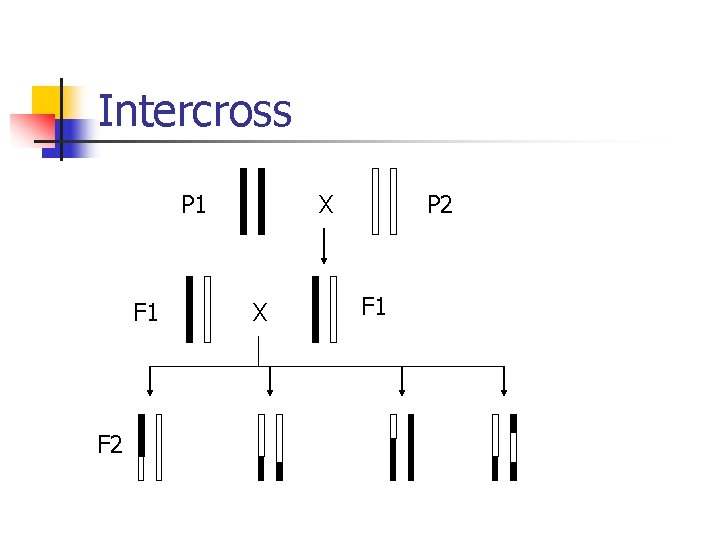
Intercross P 1 F 2 X X P 2 F 1

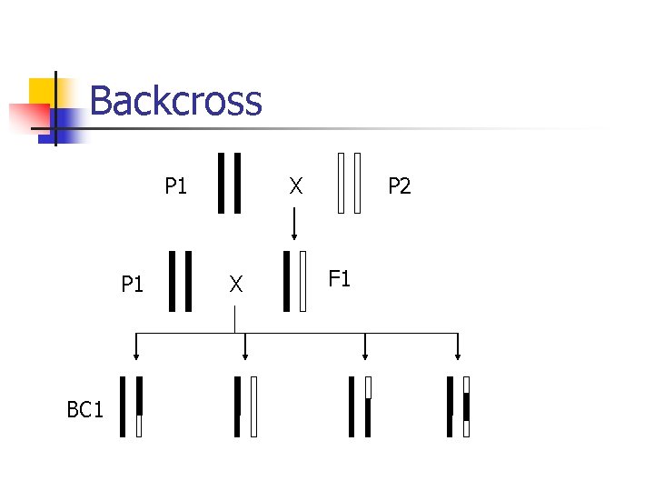
Backcross P 1 BC 1 X X P 2 F 1

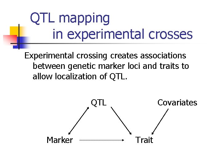
QTL mapping in experimental crosses Experimental crossing creates associations between genetic marker loci and traits to allow localization of QTL Marker Covariates Trait

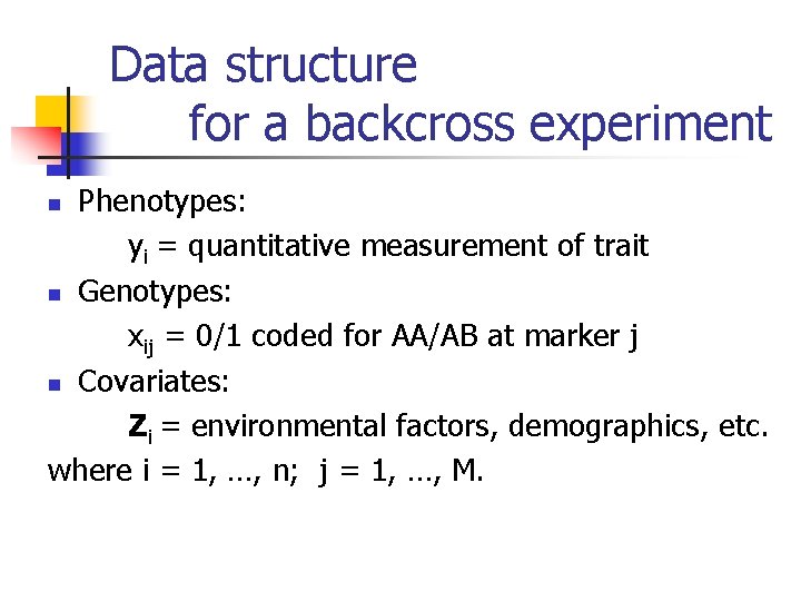
Data structure for a backcross experiment Phenotypes: yi = quantitative measurement of trait n Genotypes: xij = 0/1 coded for AA/AB at marker j n Covariates: Zi = environmental factors, demographics, etc. where i = 1, …, n; j = 1, …, M. n

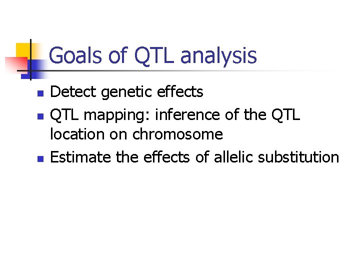
Goals of QTL analysis n n n Detect genetic effects QTL mapping: inference of the QTL location on chromosome Estimate the effects of allelic substitution

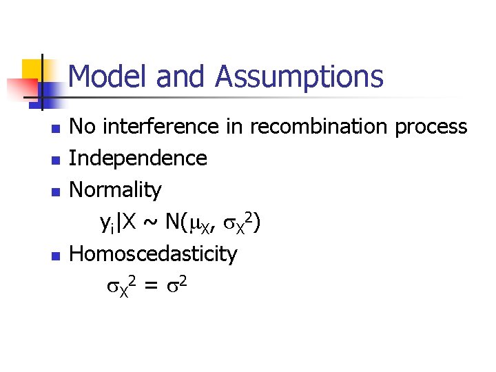
Model and Assumptions n n No interference in recombination process Independence Normality yi|X ~ N( X, X 2) Homoscedasticity X 2 = 2

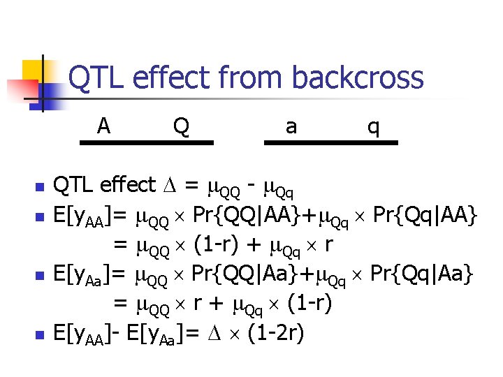
QTL effect from backcross A n n Q a q QTL effect = QQ - Qq E[y. AA]= QQ Pr{QQ|AA}+ Qq Pr{Qq|AA} = QQ (1 -r) + Qq r E[y. Aa]= QQ Pr{QQ|Aa}+ Qq Pr{Qq|Aa} = QQ r + Qq (1 -r) E[y. AA]- E[y. Aa]= (1 -2 r)

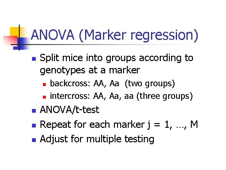
ANOVA (Marker regression) n Split mice into groups according to genotypes at a marker n n n backcross: AA, Aa (two groups) intercross: AA, Aa, aa (three groups) ANOVA/t-test Repeat for each marker j = 1, …, M Adjust for multiple testing

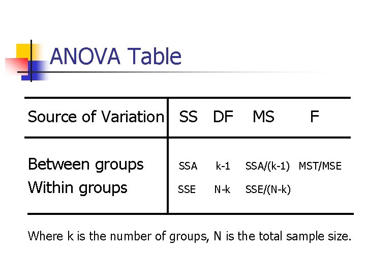
ANOVA Table Source of Variation SS DF Between groups Within groups MS F SSA k-1 SSA/(k-1) MST/MSE SSE N-k SSE/(N-k) Where k is the number of groups, N is the total sample size.

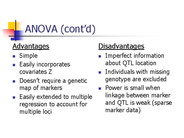
ANOVA (cont’d) Advantages n n Simple Easily incorporates covariates Z Doesn’t require a genetic map of markers Easily extended to multiple regression to account for multiple loci Disadvantages n n n Imperfect information about QTL location Individuals with missing genotype are excluded Power is small when linkage between marker and QTL is weak (sparse marker data)

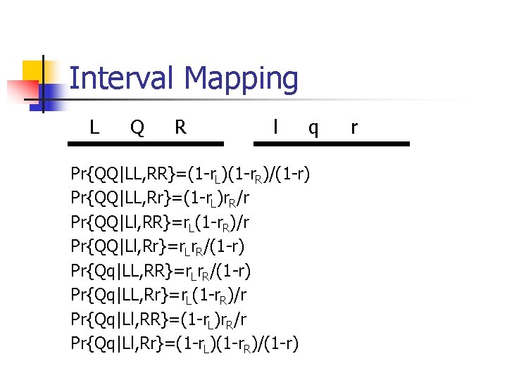
Interval Mapping L Q R l q Pr{QQ|LL, RR}=(1 -r. L)(1 -r. R)/(1 -r) Pr{QQ|LL, Rr}=(1 -r. L)r. R/r Pr{QQ|Ll, RR}=r. L(1 -r. R)/r Pr{QQ|Ll, Rr}=r. Lr. R/(1 -r) Pr{Qq|LL, RR}=r. Lr. R/(1 -r) Pr{Qq|LL, Rr}=r. L(1 -r. R)/r Pr{Qq|Ll, RR}=(1 -r. L)r. R/r Pr{Qq|Ll, Rr}=(1 -r. L)(1 -r. R)/(1 -r) r

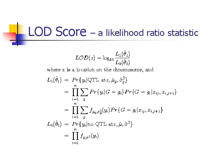
LOD Score – a likelihood ratio statistic

LOD curve n n n Likelihood profile A clear peak is taken as the QTL 1. 5 -LOD support interval

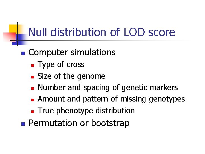
Null distribution of LOD score n Computer simulations n n n Type of cross Size of the genome Number and spacing of genetic markers Amount and pattern of missing genotypes True phenotype distribution Permutation or bootstrap

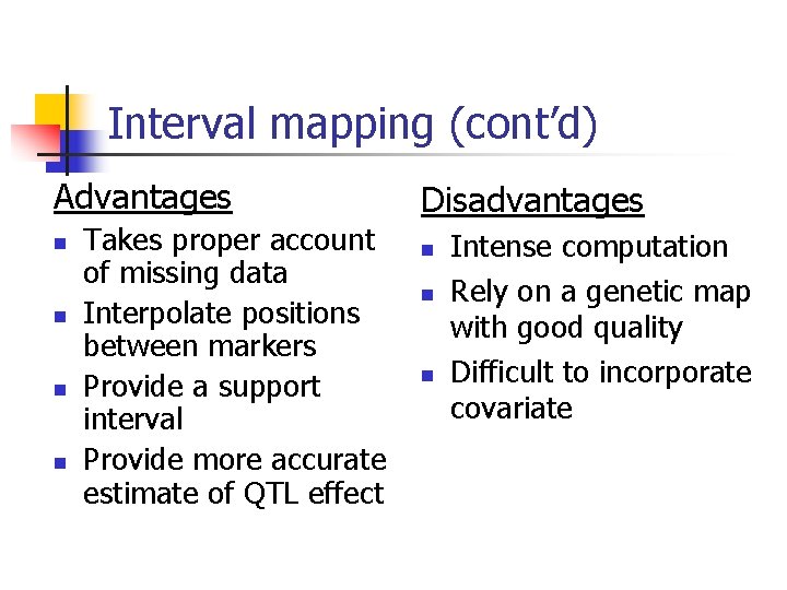
Interval mapping (cont’d) Advantages n n Takes proper account of missing data Interpolate positions between markers Provide a support interval Provide more accurate estimate of QTL effect Disadvantages n n n Intense computation Rely on a genetic map with good quality Difficult to incorporate covariate

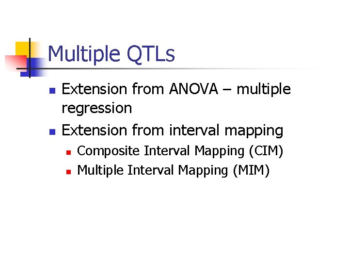
Multiple QTLs n n Extension from ANOVA – multiple regression Extension from interval mapping n n Composite Interval Mapping (CIM) Multiple Interval Mapping (MIM)

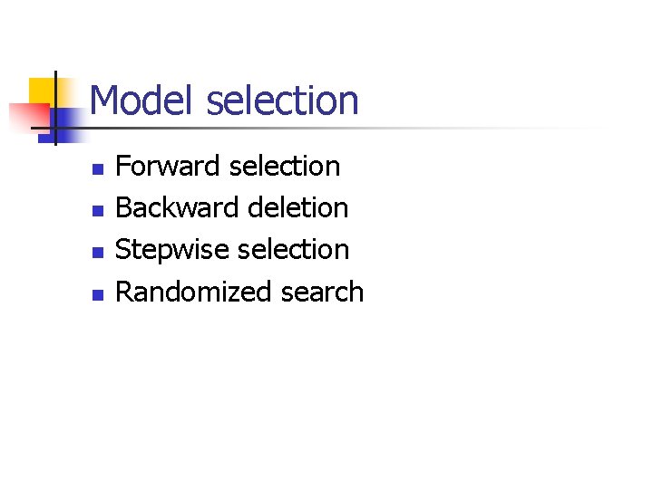
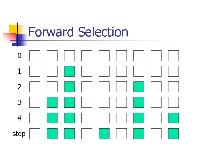
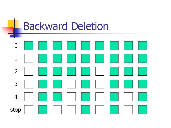
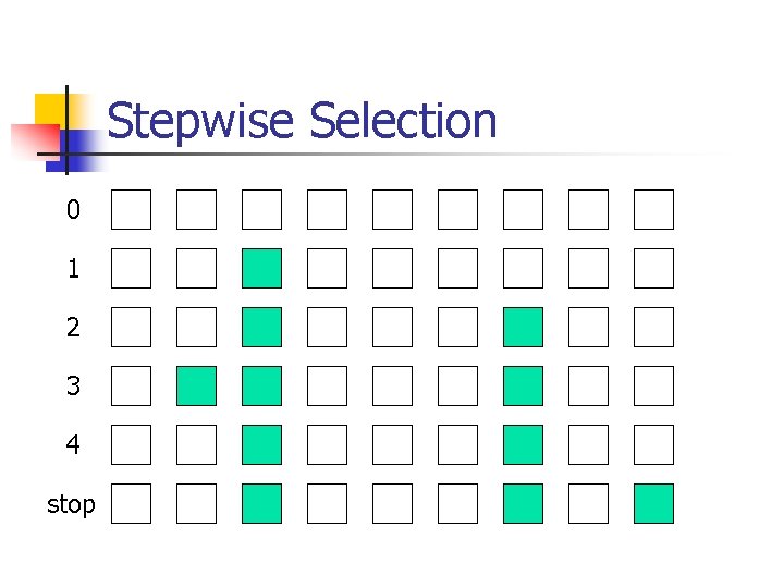
Model selection n n Forward selection Backward deletion Stepwise selection Randomized search

Forward Selection 0 1 2 3 4 stop

Backward Deletion 0 1 2 3 4 stop

Stepwise Selection 0 1 2 3 4 stop

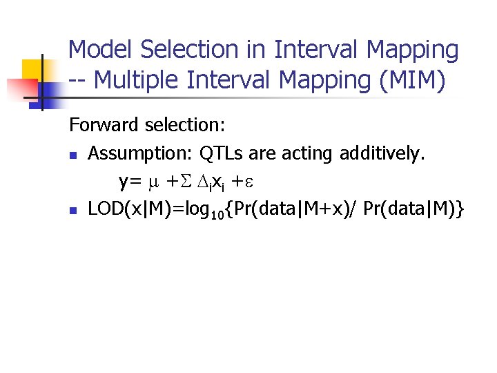
Model Selection in Interval Mapping -- Multiple Interval Mapping (MIM) Forward selection: n Assumption: QTLs are acting additively. y= + ixi + n LOD(x|M)=log 10{Pr(data|M+x)/ Pr(data|M)}

Thank you!