MIS 644 Social Newtork Analysis 20172018 Spring Chapter

MIS 644 Social Newtork Analysis 2017/2018 Spring Chapter 3 Measures and Metrics 1

Outline n Centrality Measures n Structural Balance n Similarity n Homophily and Assortative Mixing 2

n n n Structure of a network – calculate verious useful quantities or measures capture features of the topology of the network 3

Centrality Meadures n Centrality Measures n Degree n Eigen value n Katz n Closeness n Betweenness 4

Centrality Mesures n Which are the most important or central vertices in a network? n many possible definitions of importance 5

Degree Centrality n n n undirected networks – degree directed networks – in-degree and out-degree E. g. : n SNs: individuals with high connections have more prestige, access to information resources n Citation networks: papers with high in-degree, are cited more influencial papers n 6

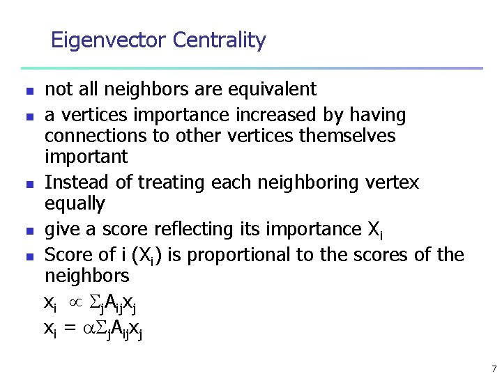
Eigenvector Centrality n n not all neighbors are equivalent a vertices importance increased by having connections to other vertices themselves important Instead of treating each neighboring vertex equally give a score reflecting its importance Xi Score of i (Xi) is proportional to the scores of the neighbors xi j. Aijxj xi = j. Aijxj 7

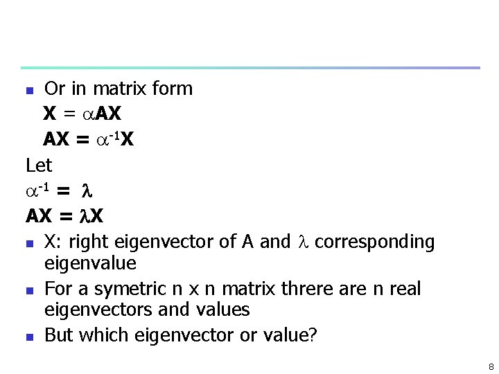
Or in matrix form X = AX AX = -1 X Let -1 = AX = X n X: right eigenvector of A and corresponding eigenvalue n For a symetric n x n matrix threre are n real eigenvectors and values n But which eigenvector or value? n 8

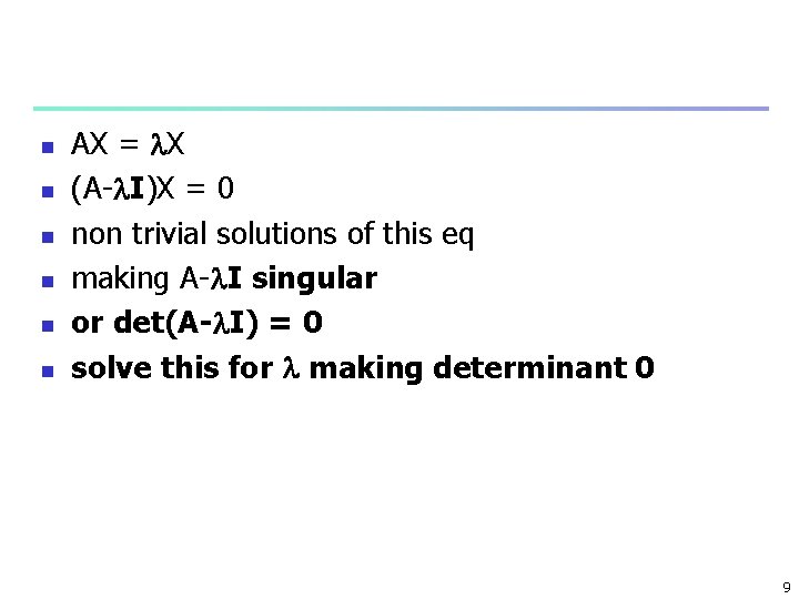
n n n AX = X (A- I)X = 0 non trivial solutions of this eq making A- I singular or det(A- I) = 0 solve this for making determinant 0 9

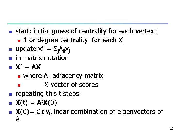
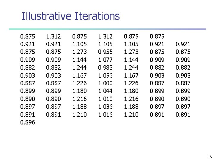
n n n n start: initial guess of centrality for each vertex i n 1 or degree centrality for each X i update x’i = j. Aijxj in matrix notation X’ = AX n where A: adjacency matrix n X vector of scores repeating this t steps: X(t) = At. X(0)= jcivi, linear combination of eigenvectors of A 10

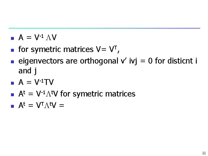
n n n A = V-1 V for symetric matrices V= VT, eigenvectors are orthogonal v’ ivj = 0 for disticnt i and j A = V-1 TV At = V-1 t. V for symetric matrices A t = V T t V = 11

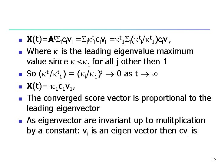
n n n X(t)=At icivi = i ticivi = t 1 i( ti/ t 1)civi, Where i is the leading eigenvalue maximum value since i< 1 for all j other then 1 So ( ti/ t 1) = ( i/ 1)t 0 as t X(t)= 1 c 1 v 1, The converged score vector is proportional to the leading eigenvector As eigenvector are invariant up to mulitplication by a constant: vi is an eigen vector then cvi is 12

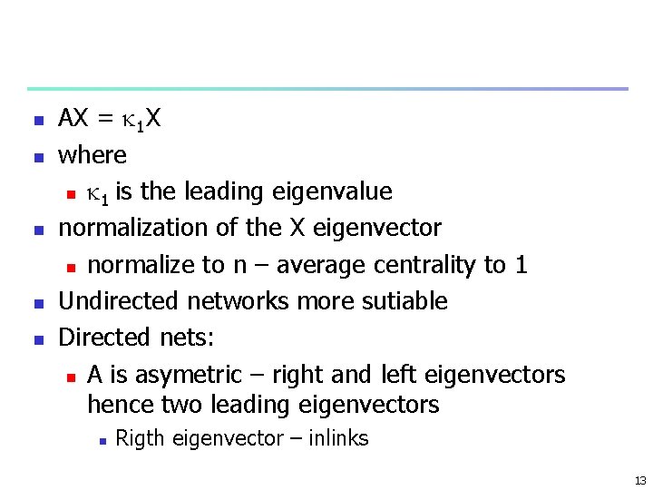
n n n AX = 1 X where n 1 is the leading eigenvalue normalization of the X eigenvector n normalize to n – average centrality to 1 Undirected networks more sutiable Directed nets: n A is asymetric – right and left eigenvectors hence two leading eigenvectors n Rigth eigenvector – inlinks 13

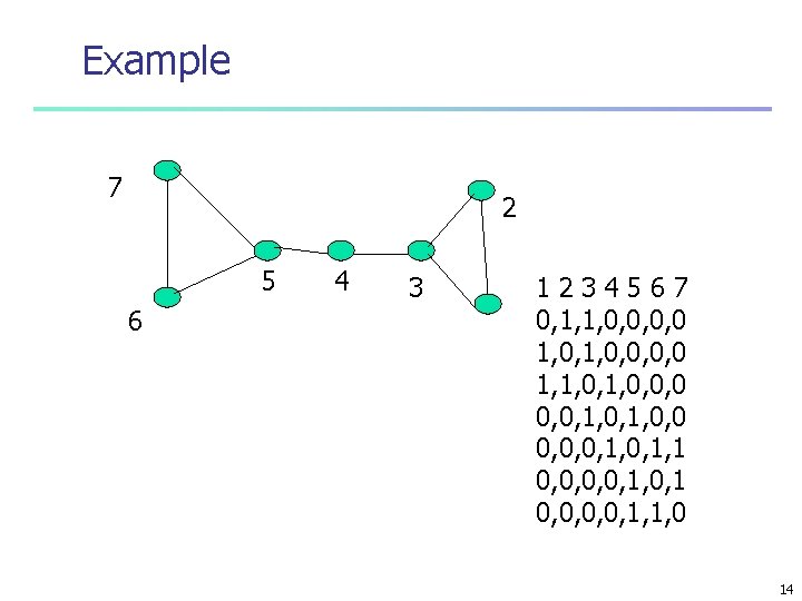
Example 7 2 5 6 4 3 1234567 0, 1, 1, 0, 0, 0, 0 1, 1, 0, 0, 0, 1, 0, 0, 0, 1, 1 0, 0, 1, 0, 1 0, 0, 1, 1, 0 14

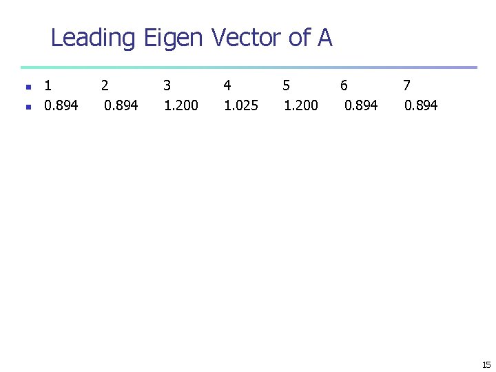
Leading Eigen Vector of A n n 1 0. 894 2 0. 894 3 1. 200 4 1. 025 5 1. 200 6 0. 894 7 0. 894 15

Illustrative Iterations 0. 875 0. 921 0. 875 0. 909 0. 882 0. 903 0. 887 0. 899 0. 890 0. 897 0. 891 0. 896 1. 312 0. 921 0. 875 0. 909 0. 882 0. 903 0. 887 0. 899 0. 890 0. 897 0. 891 0. 875 1. 105 1. 273 1. 144 1. 244 1. 167 1. 226 1. 180 1. 216 1. 188 1. 210 1. 312 1. 105 0. 955 1. 077 0. 983 1. 056 1. 000 1. 044 1. 010 1. 036 1. 016 0. 875 1. 105 1. 273 1. 144 1. 244 1. 167 1. 226 1. 180 1. 216 1. 188 1. 210 0. 875 0. 921 0. 875 0. 909 0. 882 0. 903 0. 887 0. 899 0. 890 0. 897 0. 891 16

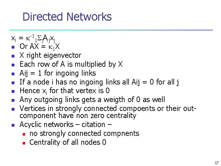
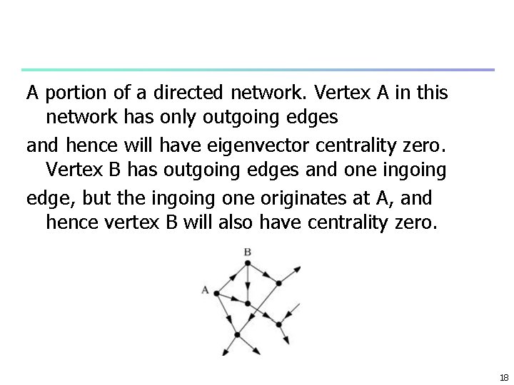
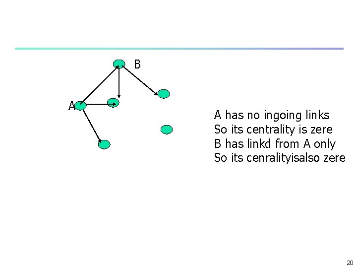
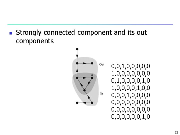
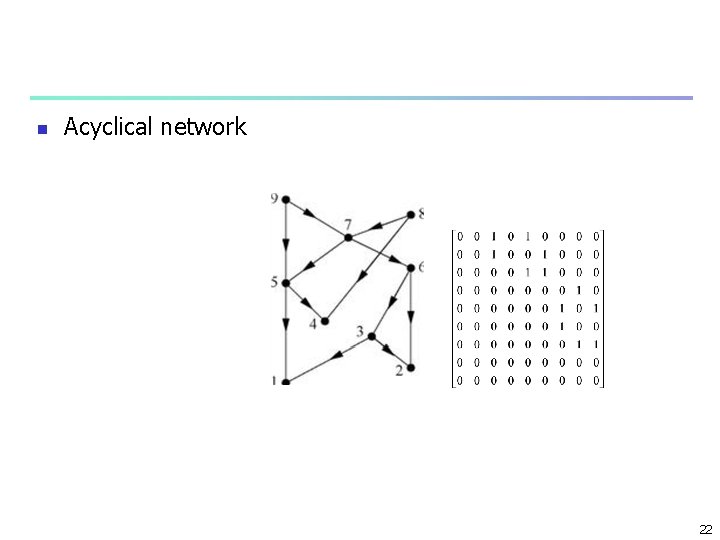
Directed Networks xi = -11 j. Aijxj n Or AX = 1 X n X right eigenvector n Each row of A is multiplied by X n Aij = 1 for ingoing links n If a node i has no ingoing links all Aij = 0 for all j n Hence xi for that vertex is 0 n Any outgoing links gets a weigth of 0 as well n Vertices in strongly connected compoents or their outcomponent have non zero centrality n Acyclic networks – citation – n no strongly connected compnents n Centrality of all nodes 0 17

A portion of a directed network. Vertex A in this network has only outgoing edges and hence will have eigenvector centrality zero. Vertex B has outgoing edges and one ingoing edge, but the ingoing one originates at A, and hence vertex B will also have centrality zero. 18

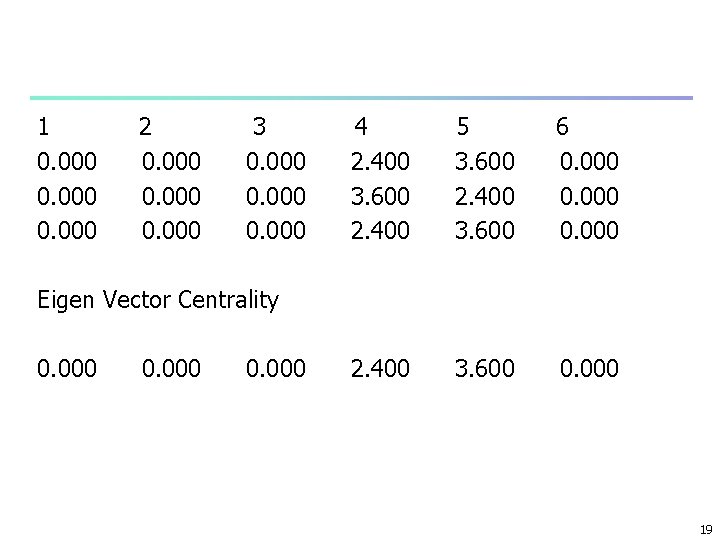
1 0. 000 2 0. 000 3 0. 000 4 2. 400 3. 600 2. 400 5 3. 600 2. 400 3. 600 6 0. 000 2. 400 3. 600 0. 000 Eigen Vector Centrality 0. 000 19

B A A has no ingoing links So its centrality is zere B has linkd from A only So its cenralityisalso zere 20

n Strongly connected component and its out components 0, 0, 1, 0, 0, 0, 0 0, 1, 0, 0, 1, 0, 0, 0, 1, 0, 0, 0, 0 0, 0, 0, 1, 0 21

n Acyclical network 22

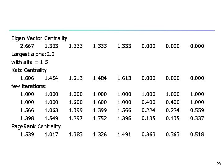
Eigen Vector Centrality 2. 667 1. 333 Largest alpha: 2. 0 with alfa = 1. 5 Katz Centrality 1. 806 1. 484 1. 613 few iterations: 1. 000 1. 600 1. 566 1. 063 1. 399 1. 398 1. 549 1. 297 Page. Rank Centrality 1. 539 1. 017 1. 383 1. 333 0. 000 1. 484 1. 613 0. 000 1. 600 1. 399 1. 752 1. 000 1. 566 1. 398 1. 000 0. 400 0. 224 0. 135 1. 000 0. 559 0. 337 1. 326 1. 491 0. 363 0. 518 23

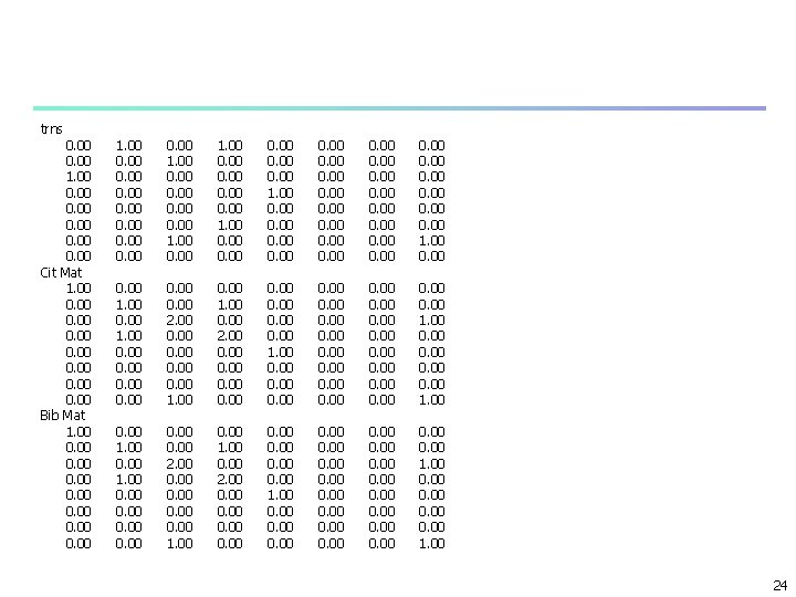
trns 0. 00 1. 00 0. 00 Cit Mat 1. 00 0. 00 Bib Mat 1. 00 0. 00 1. 00 0. 00 0. 00 0. 00 1. 00 0. 00 0. 00 2. 00 0. 00 1. 00 0. 00 2. 00 0. 00 1. 00 0. 00 0. 00 0. 00 1. 00 24

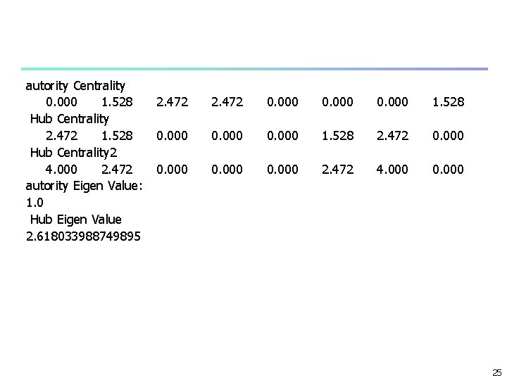
autority Centrality 0. 000 1. 528 Hub Centrality 2. 472 1. 528 Hub Centrality 2 4. 000 2. 472 autority Eigen Value: 1. 0 Hub Eigen Value 2. 618033988749895 2. 472 0. 000 1. 528 2. 472 0. 000 2. 472 4. 000 0. 000 25

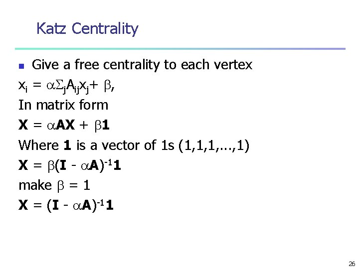
Katz Centrality Give a free centrality to each vertex xi = j. Aijxj+ , In matrix form X = AX + 1 Where 1 is a vector of 1 s (1, 1, 1, . . . , 1) X = (I - A)-11 make = 1 X = (I - A)-11 n 26

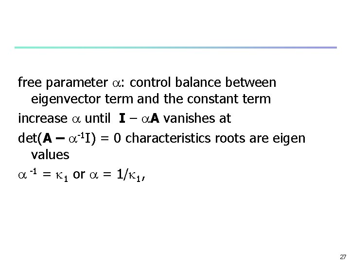
free parameter : control balance between eigenvector term and the constant term increase until I – A vanishes at det(A – -1 I) = 0 characteristics roots are eigen values -1 = 1 or = 1/ 1, 27

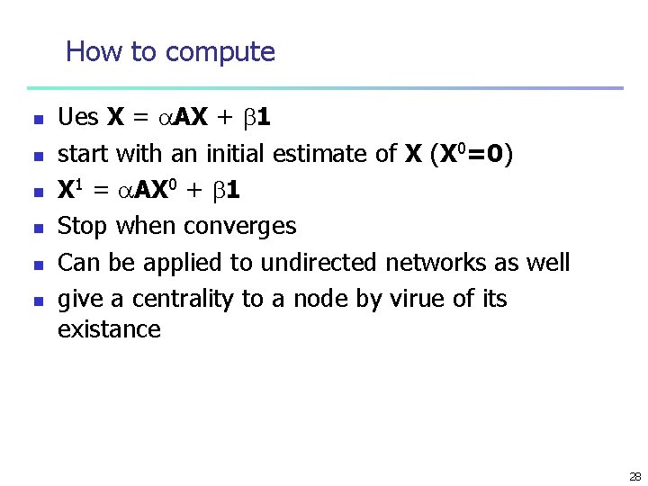
How to compute n n n Ues X = AX + 1 start with an initial estimate of X (X 0=0) X 1 = AX 0 + 1 Stop when converges Can be applied to undirected networks as well give a centrality to a node by virue of its existance 28

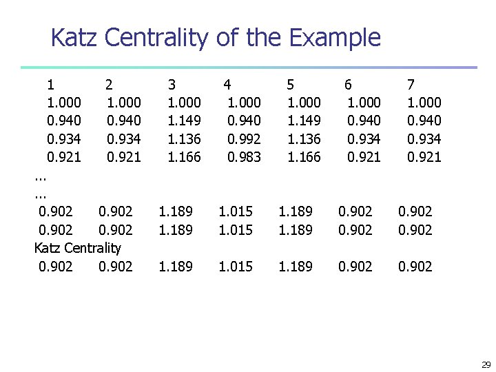
Katz Centrality of the Example 1 1. 000 0. 940 0. 934 0. 921 2 1. 000 0. 940 0. 934 0. 921 . . . 0. 902 Katz Centrality 0. 902 3 1. 000 1. 149 1. 136 1. 166 4 1. 000 0. 940 0. 992 0. 983 5 1. 000 1. 149 1. 136 1. 166 6 1. 000 0. 940 0. 934 0. 921 7 1. 000 0. 940 0. 934 0. 921 1. 189 1. 015 1. 189 0. 902 1. 189 1. 015 1. 189 0. 902 29

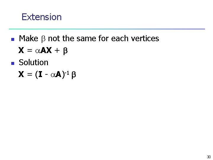
Extension n n Make not the same for each vertices X = AX + Solution X = (I - A)-1 30

Page. Rank n n n Problem with Kazt if a vertex with high Katz centrality points to another vertex those others get high centrality Yahoo high centrality if points me should my page has the high centralyity as well 31

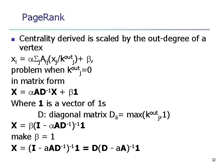
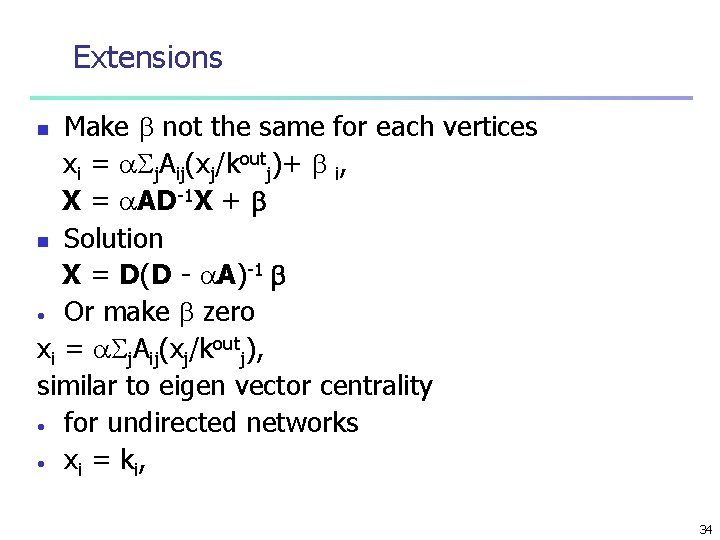
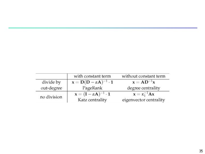
Page. Rank Centrality derived is scaled by the out-degree of a vertex xi = j. Aij(xj/koutj)+ , problem when koutj=0 in matrix form X = AD-1 X + 1 Where 1 is a vector of 1 s D: diagonal matrix Dii= max(koutj, 1) X = (I - AD-1)-11 make = 1 X = (I - a. AD-1)-11 = D(D - a. A)-11 n 32

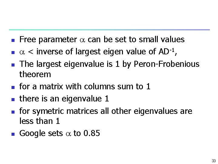
n n n n Free parameter can be set to small values < inverse of largest eigen value of AD-1, The largest eigenvalue is 1 by Peron-Frobenious theorem for a matrix with columns sum to 1 there is an eigenvalue 1 for symetric matrices all other eigenvalues are less than 1 Google sets to 0. 85 33

Extensions Make not the same for each vertices xi = j. Aij(xj/koutj)+ i, X = AD-1 X + n Solution X = D(D - A)-1 • Or make zero xi = j. Aij(xj/koutj), similar to eigen vector centrality • for undirected networks • xi = k i , n 34

35

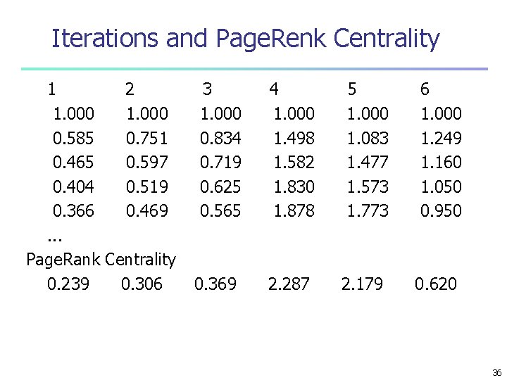
Iterations and Page. Renk Centrality 1 2 1. 000 0. 585 0. 751 0. 465 0. 597 0. 404 0. 519 0. 366 0. 469. . . Page. Rank Centrality 0. 239 0. 306 3 1. 000 0. 834 0. 719 0. 625 0. 565 0. 369 4 1. 000 1. 498 1. 582 1. 830 1. 878 2. 287 5 1. 000 1. 083 1. 477 1. 573 1. 773 2. 179 6 1. 000 1. 249 1. 160 1. 050 0. 950 0. 620 36

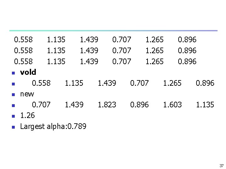
0. 558 1. 135 1. 439 0. 707 1. 265 0. 896 n vold n 0. 558 1. 135 1. 439 0. 707 1. 265 0. 896 n new n 0. 707 1. 439 1. 823 0. 896 1. 603 1. 135 n 1. 26 n Largest alpha: 0. 789 37

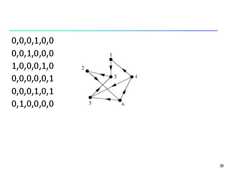
0, 0, 0, 1, 0, 0, 0, 1, 0 0, 0, 0, 1 0, 1, 0, 0 38

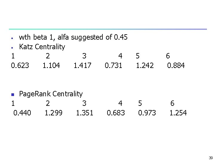
wth beta 1, alfa suggested of 0. 45 • Katz Centrality 1 2 3 4 0. 623 1. 104 1. 417 0. 731 • Page. Rank Centrality 1 2 3 0. 440 1. 299 1. 351 5 1. 242 6 0. 884 n 4 0. 683 5 0. 973 6 1. 254 39

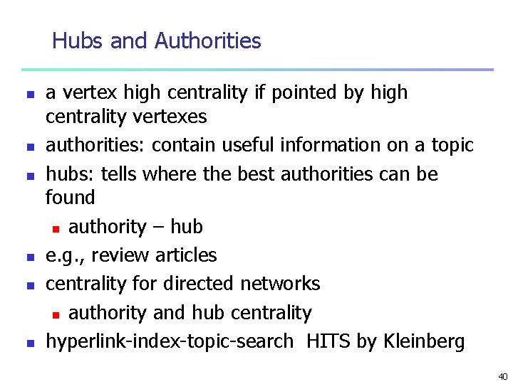
Hubs and Authorities n n n a vertex high centrality if pointed by high centrality vertexes authorities: contain useful information on a topic hubs: tells where the best authorities can be found n authority – hub e. g. , review articles centrality for directed networks n authority and hub centrality hyperlink-index-topic-search HITS by Kleinberg 40

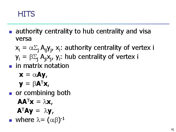
HITS n n authority centrality to hub centrality and visa versa xi = j Aijyj, xi: authority centrality of vertex i yi = j Ajixj, yi: hub centrality of vertex i in matrix notation x = Ay, y = ATx, or combining both AATx = x, ATAy = y, where = ( )-1 41

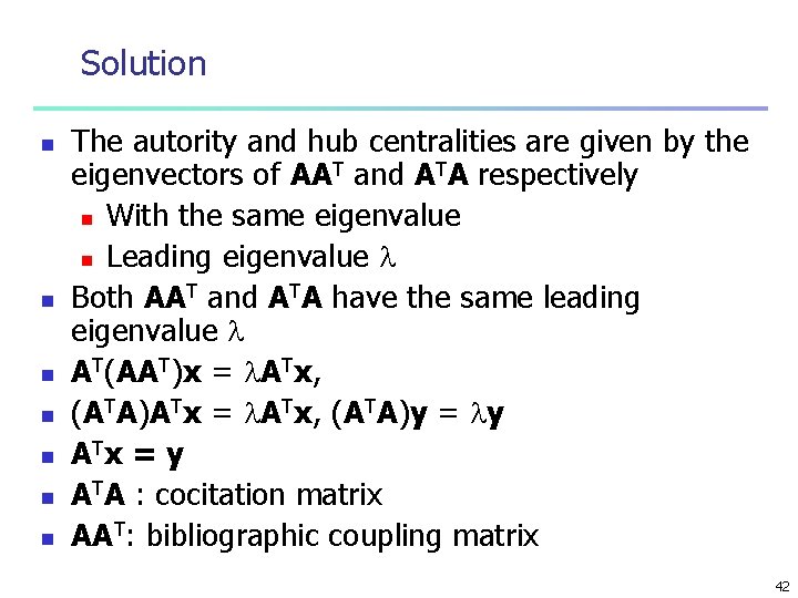
Solution n n n The autority and hub centralities are given by the eigenvectors of AAT and ATA respectively n With the same eigenvalue n Leading eigenvalue Both AAT and ATA have the same leading eigenvalue AT(AAT)x = ATx, (ATA)ATx = ATx, (ATA)y = y ATx = y ATA : cocitation matrix AAT: bibliographic coupling matrix 42

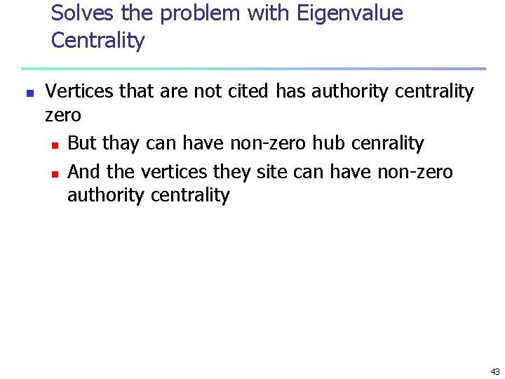
Solves the problem with Eigenvalue Centrality n Vertices that are not cited has authority centrality zero n But thay can have non-zero hub cenrality n And the vertices they site can have non-zero authority centrality 43

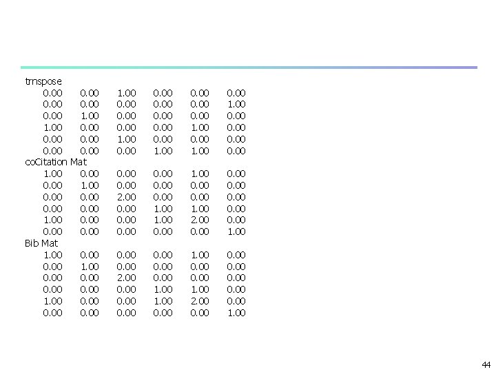
trnspose 0. 00 1. 00 0. 00 co. Citation Mat 1. 00 0. 00 1. 00 0. 00 Bib Mat 1. 00 0. 00 0. 00 1. 00 0. 00 2. 00 0. 00 1. 00 0. 00 1. 00 2. 00 0. 00 1. 00 44

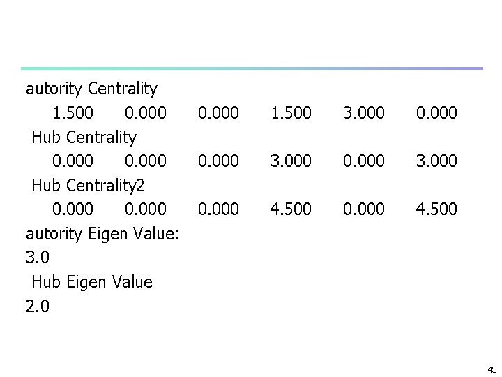
autority Centrality 1. 500 0. 000 Hub Centrality 2 0. 000 autority Eigen Value: 3. 0 Hub Eigen Value 2. 0 0. 000 1. 500 3. 000 0. 000 4. 500 0. 000 4. 500 45

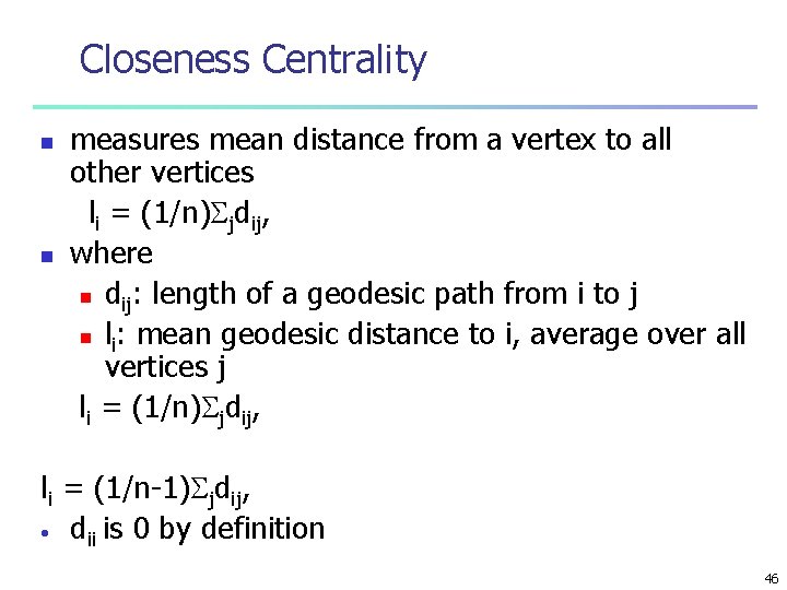
Closeness Centrality n n measures mean distance from a vertex to all other vertices li = (1/n) jdij, where n dij: length of a geodesic path from i to j n li: mean geodesic distance to i, average over all vertices j li = (1/n) jdij, li = (1/n-1) jdij, • dii is 0 by definition 46

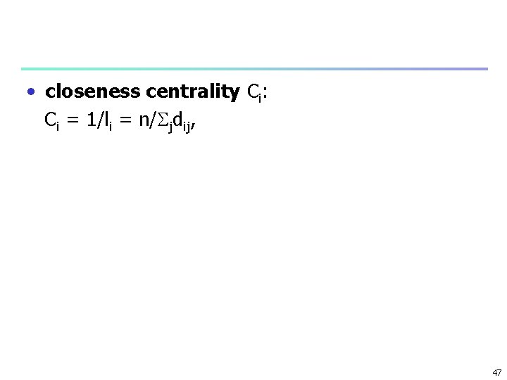
• closeness centrality Ci: Ci = 1/li = n/ jdij, 47

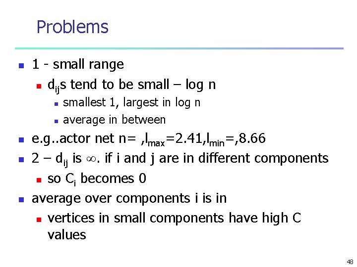
Problems n 1 - small range n dijs tend to be small – log n n n smallest 1, largest in log n average in between e. g. . actor net n= , lmax=2. 41, lmin=, 8. 66 2 – dij is . if i and j are in different components n so Ci becomes 0 average over components i is in n vertices in small components have high C values 48

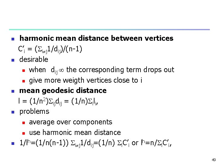
n n n harmonic mean distance between vertices C’i = ( i j 1/dij)/(n-1) desirable n when dij the corresponding term drops out n give more weigth vertices close to i mean geodesic distance l = (1/n 2) ijdij = (1/n) ili, problems n average over components n use harmonic mean distance 1/lh=(1/n(n-1)) i j 1/dij=(1/n) i. C’i or lh=n/ i. C’i, 49

Betweenness Centrality n n the extend to which a vertex lies on paths between other vertices the number of geodesic paths the vertex lies on betweenness centrality or betweenness high influence n control of information passing to others n removel most disrupt communication 50

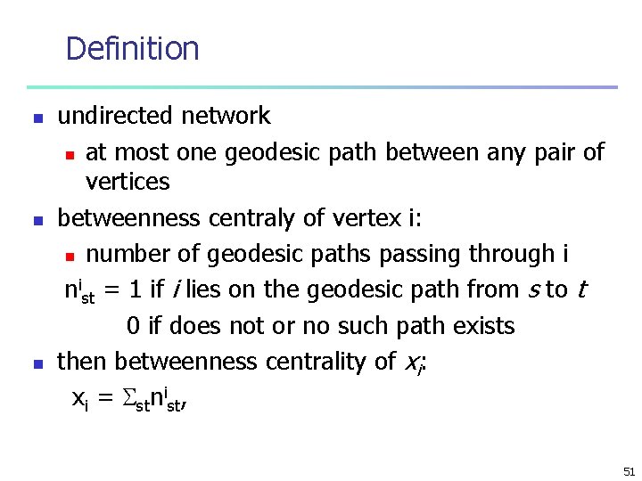
Definition n undirected network n at most one geodesic path between any pair of vertices betweenness centraly of vertex i: n number of geodesic paths passing through i nist = 1 if i lies on the geodesic path from s to t 0 if does not or no such path exists then betweenness centrality of xi: xi = stnist, 51

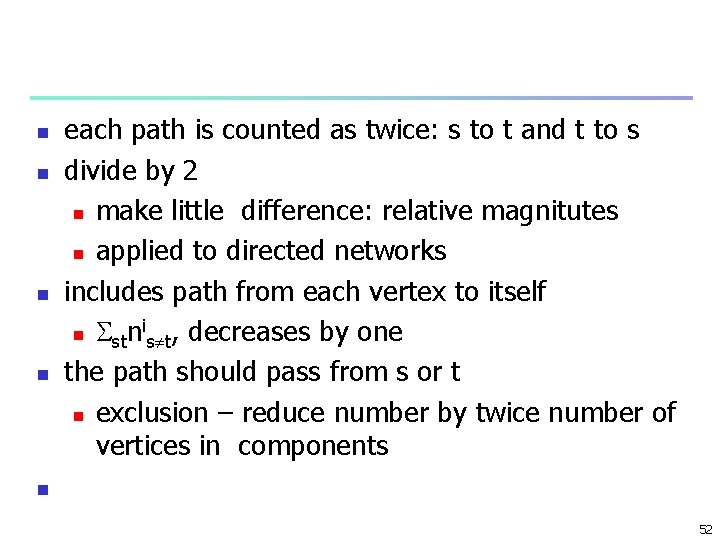
n n each path is counted as twice: s to t and t to s divide by 2 n make little difference: relative magnitutes n applied to directed networks includes path from each vertex to itself i n stn s t, decreases by one the path should pass from s or t n exclusion – reduce number by twice number of vertices in components n 52

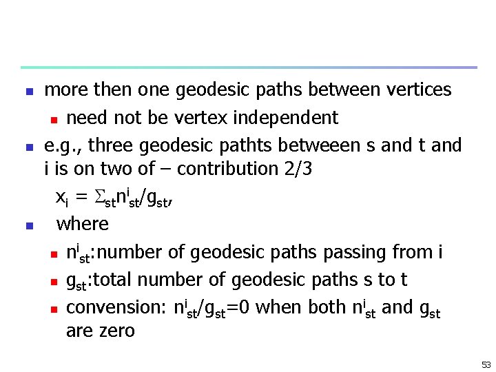
n n n more then one geodesic paths between vertices n need not be vertex independent e. g. , three geodesic pathts betweeen s and t and i is on two of – contribution 2/3 xi = stnist/gst, where i n n st: number of geodesic paths passing from i n gst: total number of geodesic paths s to t i i n convension: n st/gst=0 when both n st and gst are zero 53

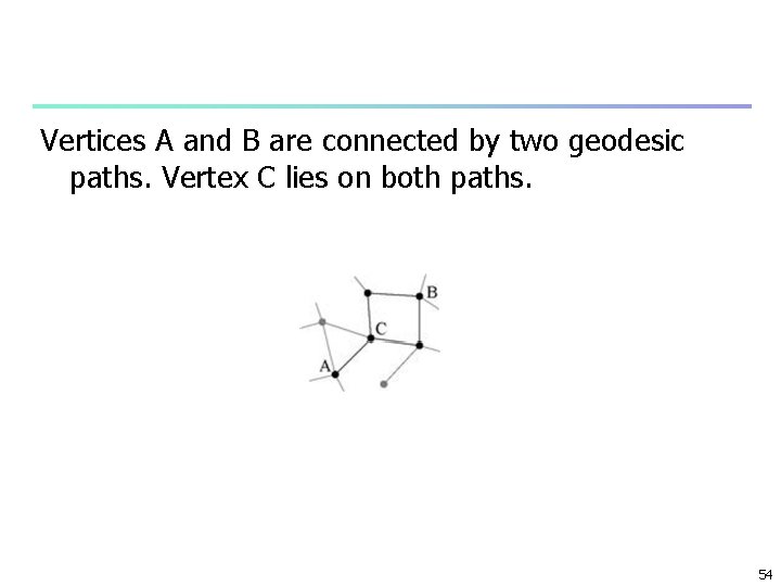
Vertices A and B are connected by two geodesic paths. Vertex C lies on both paths. 54

n n n directed networks n shortest paths depend on the direction not a measure of n how well connected a vertex is instead n how much a vertex falls between others on average, Figure 7. 2 N-N 55

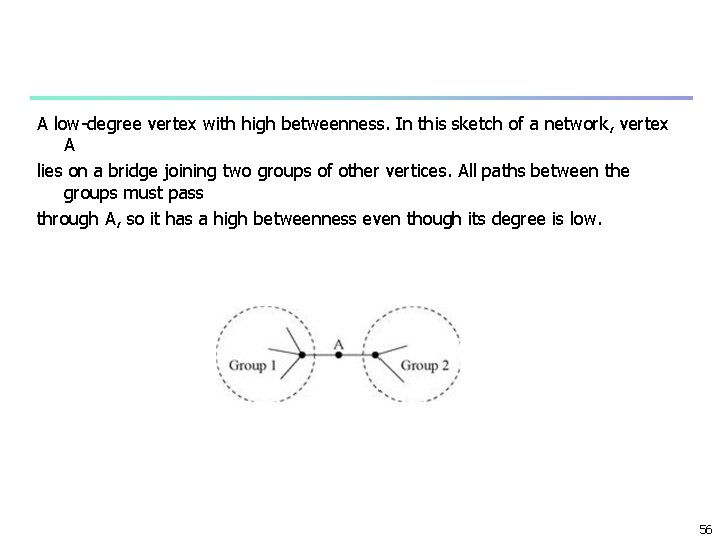
A low-degree vertex with high betweenness. In this sketch of a network, vertex A lies on a bridge joining two groups of other vertices. All paths between the groups must pass through A, so it has a high betweenness even though its degree is low. 56

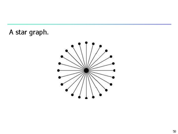
Range of values n n Values are distributed over wide range n maximum value: on the shortest path of every other vertex–center of a star n 2 -(n-1)=n 2 -n+1 n minimum value: 2(n-1)+1=2 n-1, a leaf: connected by an edge ratio of largest to smallest possible values n 2 -n+1/2 n-1 n/2, real networks ratio is not as high but still large n increases with n e. g. , film actors : 8. 91 x 105 – 7. 47 x 108, 57

A star graph. 58

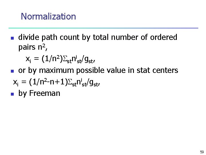
Normalization divide path count by total number of ordered pairs n 2, xi = (1/n 2) stnist/gst, n or by maximum possible value in stat centers xi = (1/n 2 -n+1) stnist/gst, n by Freeman n 59

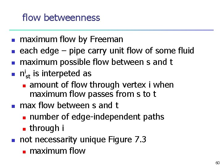
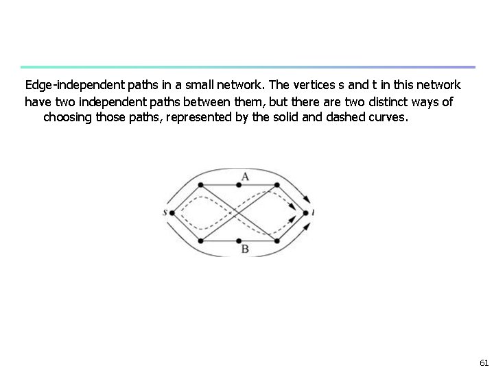
flow betweenness n n n maximum flow by Freeman each edge – pipe carry unit flow of some fluid maximum possible flow between s and t nist is interpeted as n amount of flow through vertex i when maximum flow passes from s to t max flow between s and t n number of edge-independent paths n through i not necessarity unique Figure 7. 3 n maximum flow 60

Edge-independent paths in a small network. The vertices s and t in this network have two independent paths between them, but there are two distinct ways of choosing those paths, represented by the solid and dashed curves. 61

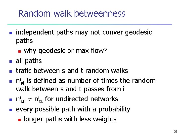
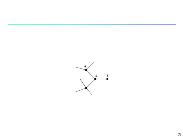
Random walk betweenness n n n independent paths may not conver geodesic paths n why geodesic or max flow? all paths trafic between s and t random walks nist is defined as number of times the random walk between s and t passes from i nist nits for undirected networks every possible path with a probability n longer paths with less weights 62

63

Groups of Vertices n n groups or communities e. g. , n networks of people n n www n n n friends, coverkers, business partners groups of related web pages sophisticated – hierachical clustering, spectral partitioning simpler – probing and describing n local structure of networks n cliques, plexes, cores and components 64

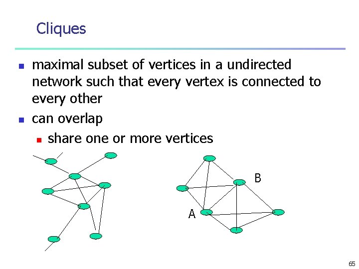
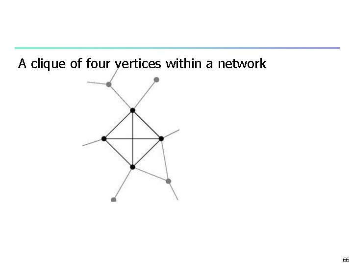
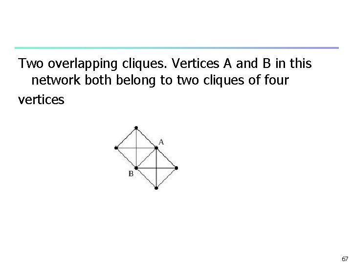
Cliques n n maximal subset of vertices in a undirected network such that every vertex is connected to every other can overlap n share one or more vertices B A 65

A clique of four vertices within a network 66

Two overlapping cliques. Vertices A and B in this network both belong to two cliques of four vertices 67

n n clique – a highly cohesive subgroup e. g. : in a SN set of individuals each of whom acquainted with each other n a set of coworkers in a office n set of classsmates in a school near cliques n some members may be unacquainted n even most are 68

k-plex n n n a k-plex of size n: maximal subset of n vertices such that every member is connected at least n-k of the others k = 1 is clique what is the value of k? n experimentation – start with small values for small groups specify percentage n each member is connected to a certain fraction of the others 69

k-core n n maximal subset of vertices such that each is connected to at least k others k-core of n vertices is (n-k)-plex cannot overlap like cliques or k-plexes An algorithm to find k-cores n start with a network n repeadly n n remove any vertex with degree less than k until no such vertex remains 70

Components and k-components n n n a k-component or k-connected component n maximal subset of vertices such that each is reachable from each of the others by at least k -vertex independent paths n k=1, ordinary component n k=2, bicomponent n k=3, tricomponent an i-component is a sub set of (i-1)-component number of vertex-independent paths equals to the size of the cut set between i and j 71

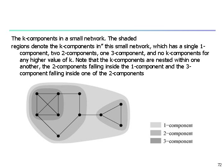
The k-components in a small network. The shaded regions denote the k-components in” this small network, which has a single 1 component, two 2 -components, one 3 -component, and no k-components for any higher value of k. Note that the k-components are nested within one another, the 2 -components falling inside the 1 -component and the 3 component falling inside one of the 2 -components 72

Network robustness n n n Internet n number of independent paths n number of independent routes size of cut set n number of routers that would have to fail or the data connection serves between the two ends k>=3 may non-contiguous k 1, 2 contiguous Figure on page 197 N-N 73

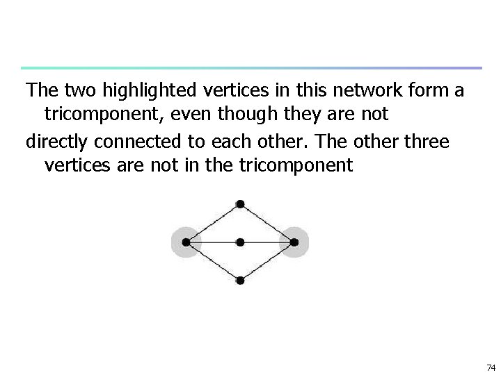
The two highlighted vertices in this network form a tricomponent, even though they are not directly connected to each other. The other three vertices are not in the tricomponent 74

Transitivity n n A relation transitive if a b and b c together implied a c e. g. , =, <, > in network analysis n connected to n n u is connect to v, v is connected to w undireceted networks – perfect transitivity n fully connected components clique partial transitivity 75

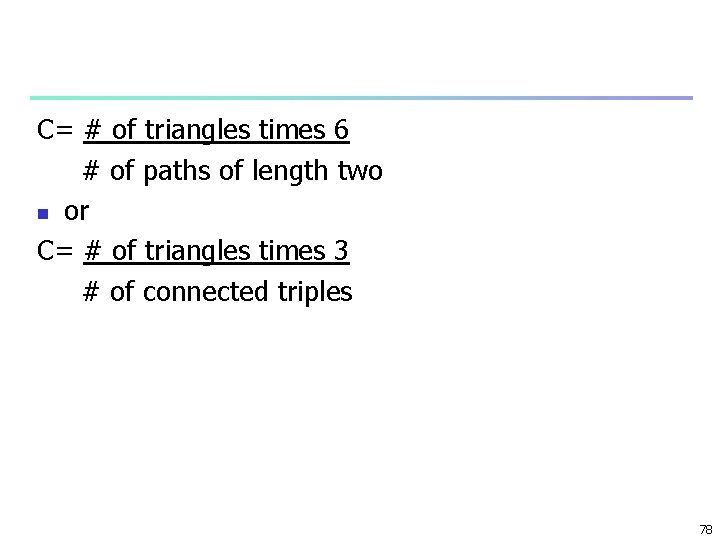
n n n u knows v and v knows w does not guarantee u knows w n but makes it much more likely if u knows v and v knows w – uvw: length 2 if u knows w as well a length 3 cycle – triad C= # of closed paths of length two # of paths of length two C=1, perfect connectivity C=0, tree, square latice, n 76

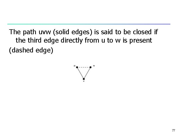
The path uvw (solid edges) is said to be closed if the third edge directly from u to w is present (dashed edge) 77

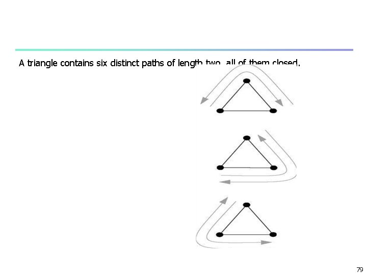
C= # of triangles times 6 # of paths of length two n or C= # of triangles times 3 # of connected triples 78

A triangle contains six distinct paths of length two, all of them closed. 79

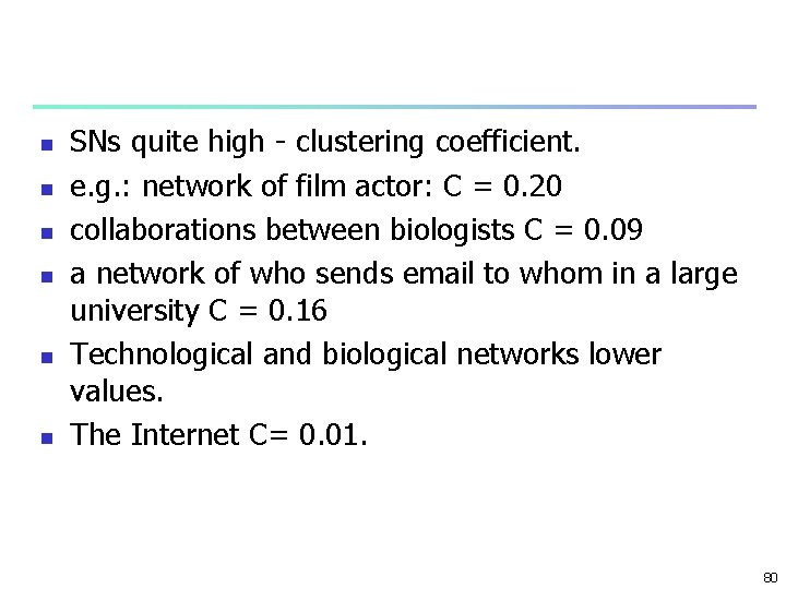
n n n SNs quite high - clustering coefficient. e. g. : network of film actor: C = 0. 20 collaborations between biologists C = 0. 09 a network of who sends email to whom in a large university C = 0. 16 Technological and biological networks lower values. The Internet C= 0. 01. 80

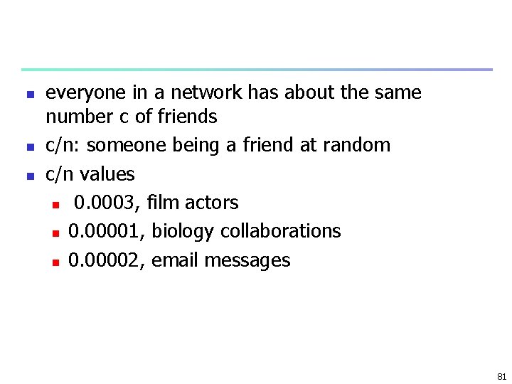
n n n everyone in a network has about the same number c of friends c/n: someone being a friend at random c/n values n 0. 0003, film actors n 0. 00001, biology collaborations n 0. 00002, email messages 81

Local Clustering and Redundency defined for vertex i Ci= # of pairs of neighbors of i that are connected # of pairs of neighbors of i n denominator: (1/2)ki(ki-1) n local clustering n emprical finding: n rough dependence on degree n higher degree lower local clustering coef. n 82

n Structural holes: n few of neighbors are connected low C i, n bad: efficient flow of intromation or trafic n good: control of infromation flow to its neighbors 83

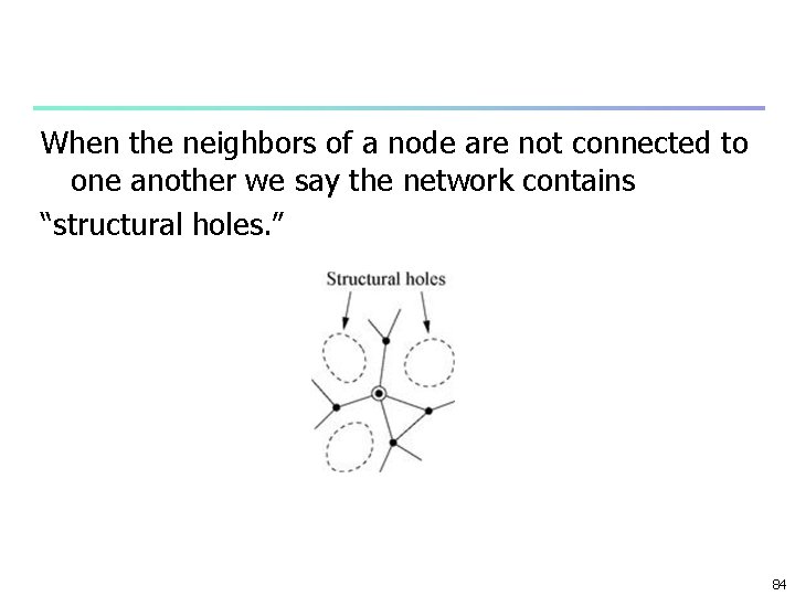
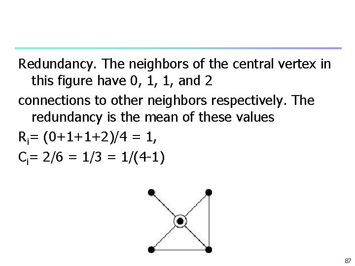
When the neighbors of a node are not connected to one another we say the network contains “structural holes. ” 84

n n local clustering n inverse of betweenness centrality n betweenness centrality – contral of flow of information all pairs of vertices in a component local clustering: n local version of betweenness n control over its neighbors 85

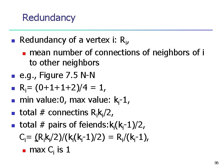
Redundancy n n n Redundancy of a vertex i: Ri, n mean number of connections of neighbors of i to other neighbors e. g. , Figure 7. 5 N-N Ri= (0+1+1+2)/4 = 1, min value: 0, max value: ki-1, total # connectins Riki/2, total # pairs of feiends: ki(ki-1)/2, Ci= (Riki/2)/(ki(ki-1)/2) = Ri/(ki-1), n max Ci is 1 86

Redundancy. The neighbors of the central vertex in this figure have 0, 1, 1, and 2 connections to other neighbors respectively. The redundancy is the mean of these values Ri= (0+1+1+2)/4 = 1, Ci= 2/6 = 1/3 = 1/(4 -1) 87

Another definition of global clustering coefficient n n n global clustering as an average of local clustering coefficients Cws = (1/n) ni=1 Ci, not the same value with other definition dominated by vertices with low degree 88

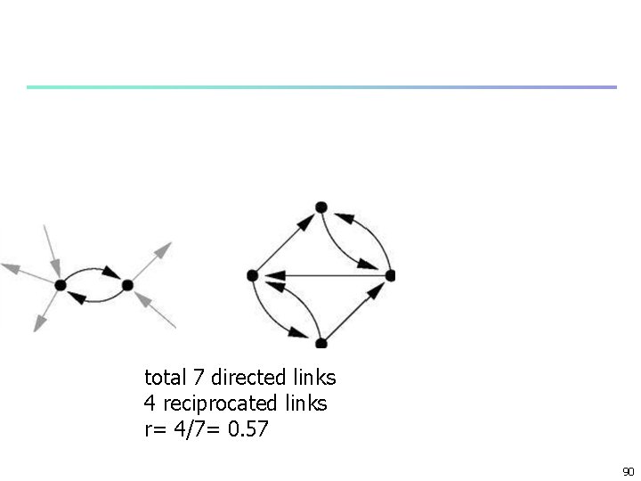
Reciprocity n n n n directed networks – shortest loops – length 2 Frequency of loops of length 2 – reciprocity e. g. , www, friendship networks link from i to j and j to i the edge is reciprocated reciprocity r defined n fraction of edges reciprocated Aij. Aji = 1, reciprocated 0 otherwise r = ij. Aji = Tr. A 2, 89

total 7 directed links 4 reciprocated links r= 4/7= 0. 57 90

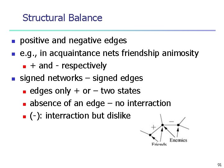
Structural Balance n n n positive and negative edges e. g. , in acquaintance nets friendship animosity n + and - respectively signed networks – signed edges n edges only + or – two states n absence of an edge – no interraction n (-): interraction but dislike 91

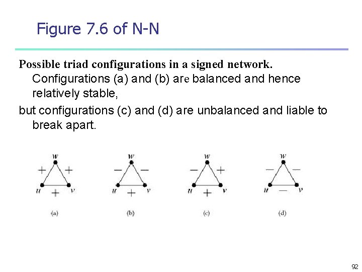
Figure 7. 6 of N-N Possible triad configurations in a signed network. Configurations (a) and (b) are balanced and hence relatively stable, but configurations (c) and (d) are unbalanced and liable to break apart. 92

n n n n (a) fine (b) animy of my animy is my friend (c) problematic. u likes v and v likes w, but u thinks w is an idiot. a strain on the friendship between u and v because u thinks v s friend is an idiot. Alternatively, from the point of view of v, v has two friends, u and w they don’t get along resolved by one of the acquaintances being broken. 93

n n n (d) somewhat ambiguous. On the one hand, it consists of three people who all dislike each other On the other hand, the “enemy of my enemy” rule does not apply cause tension. unstable. not stay together three enemies 94

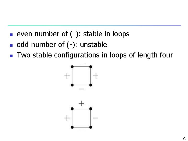
n n n even number of (-): stable in loops odd number of (-): unstable Two stable configurations in loops of length four 95

Harary Theorem n n Networks containing only loops with even numbers of minus signs are said to show structural balance, or sometimes just balance A balanced network can be divided into connected groups of vertices such that all n connections between members of the same group are positive and all connections between members of different groups are negative 96

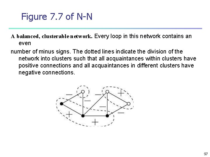
Figure 7. 7 of N-N A balanced, clusterable network. Every loop in this network contains an even number of minus signs. The dotted lines indicate the division of the network into clusters such that all acquaintances within clusters have positive connections and all acquaintances in different clusters have negative connections. 97

Constructive proof n n n 1. A vertex v connected by a positive edge to another u that has already been colored gets colored the same as u. 2. A vertex v connected by a negative edge to another u that has already been colored gets colored the opposite color from u 98

n n n come upon a vertex whose color has already been assigned possibility of a conflict network as a whole is unbalanced 99

n n n n a vertex that has already been colored in, it another path by which that vertex can be reached from our starting point possibly more than one, loop this vertex belongs— balanced networks, every loop to which our vertex belongs must have an even number of negative edges around it 100

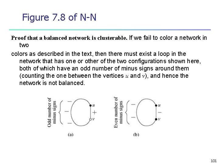
Figure 7. 8 of N-N Proof that a balanced network is clusterable. If we fail to color a network in two colors as described in the text, then there must exist a loop in the network that has one or other of the two configurations shown here, both of which have an odd number of minus signs around them (counting the one between the vertices u and v), and hence the network is not balanced. 101

n n n most social networks are in balanced or mostly balanced state n everyone likes others within their group n and dislikes those in other groups Structural balance and clusterability in networks are thus a model for cliquishness or insularity, with people tending to stick together in like-minded groups and disdaining everyone outside their immediate community. 102

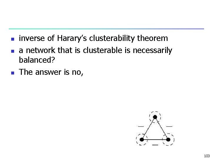
n n n inverse of Harary’s clusterability theorem a network that is clusterable is necessarily balanced? The answer is no, 103

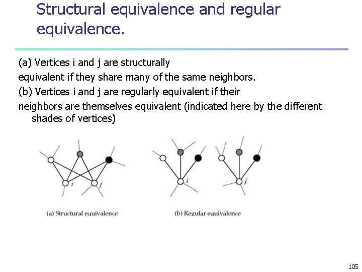
Similarity n not individual characteristics but network structure two approaches n structural equivalence n n two vertices are structurally equivlent if they share many of the same network neighbors regular equivalence n not necessarily same neighbors but neigfhbors themselfs similar 104

Structural equivalence and regular equivalence. (a) Vertices i and j are structurally equivalent if they share many of the same neighbors. (b) Vertices i and j are regularly equivalent if their neighbors are themselves equivalent (indicated here by the different shades of vertices) 105

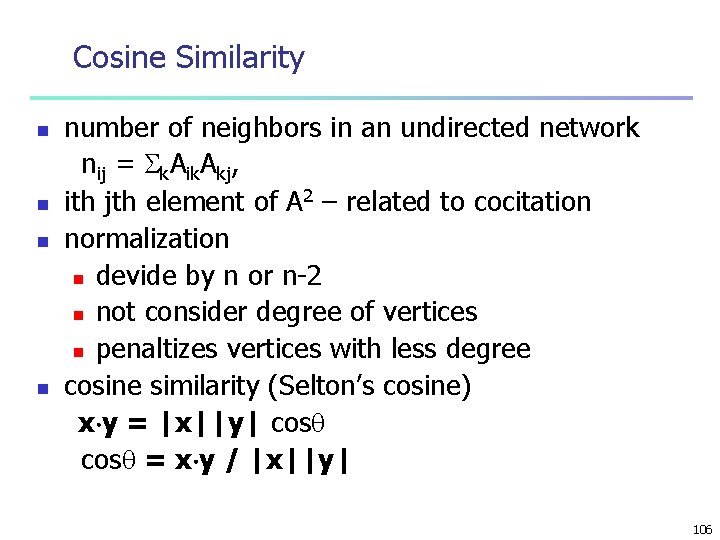
Cosine Similarity n n number of neighbors in an undirected network nij = k. Aik. Akj, ith jth element of A 2 – related to cocitation normalization n devide by n or n-2 n not consider degree of vertices n penaltizes vertices with less degree cosine similarity (Selton’s cosine) x y = |x||y| cos = x y / |x||y| 106

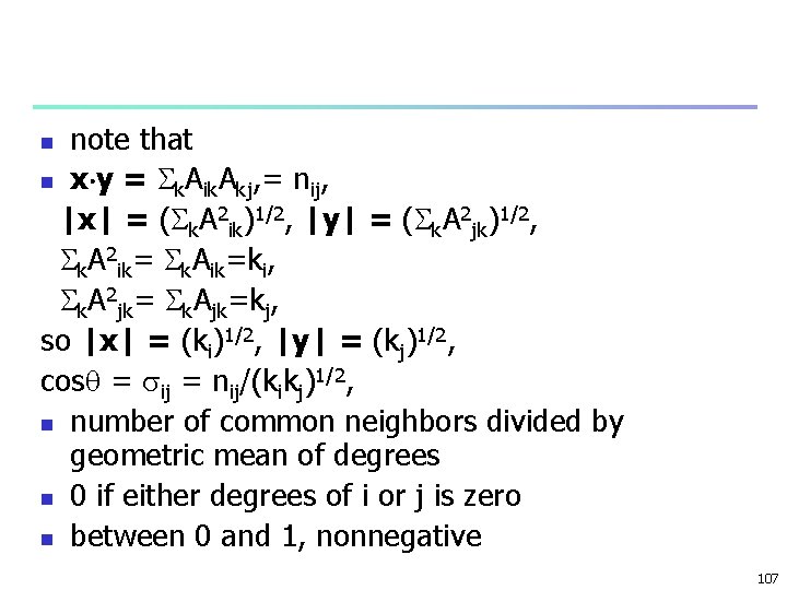
note that n x y = k. Aik. Akj, = nij, |x| = ( k. A 2 ik)1/2, |y| = ( k. A 2 jk)1/2, k. A 2 ik= k. Aik=ki, k. A 2 jk= k. Ajk=kj, so |x| = (ki)1/2, |y| = (kj)1/2, cos = ij = nij/(kikj)1/2, n number of common neighbors divided by geometric mean of degrees n 0 if either degrees of i or j is zero n between 0 and 1, nonnegative n 107

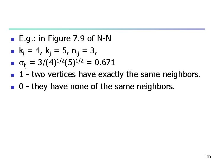
n n n E. g. : in Figure 7. 9 of N-N ki = 4, kj = 5, nij = 3, ij = 3/(4)1/2(5)1/2 = 0. 671 1 - two vertices have exactly the same neighbors. 0 - they have none of the same neighbors. 108

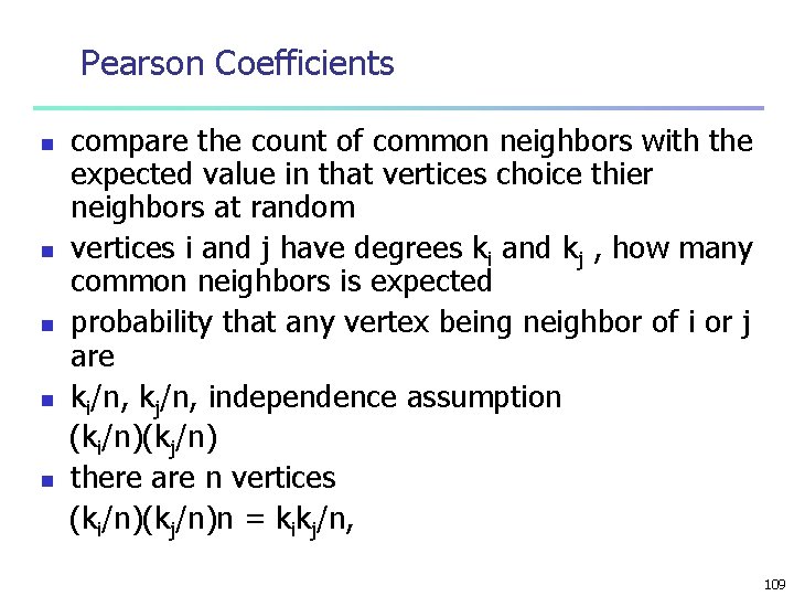
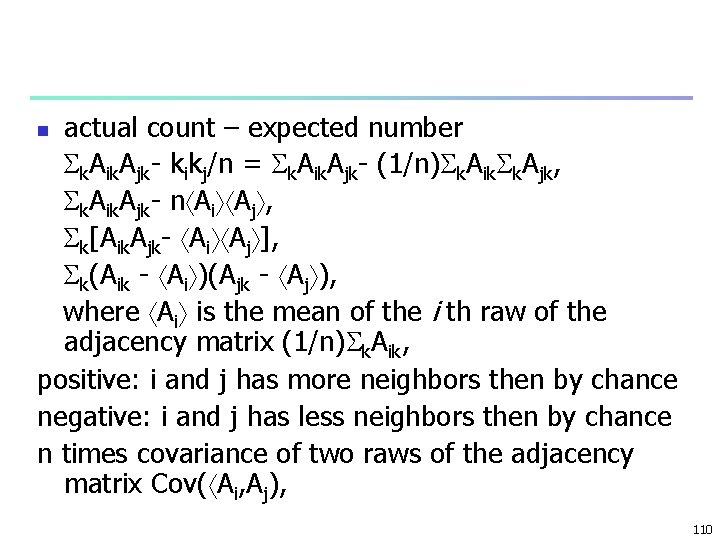
Pearson Coefficients n n n compare the count of common neighbors with the expected value in that vertices choice thier neighbors at random vertices i and j have degrees ki and kj , how many common neighbors is expected probability that any vertex being neighbor of i or j are ki/n, kj/n, independence assumption (ki/n)(kj/n) there are n vertices (ki/n)(kj/n)n = kikj/n, 109

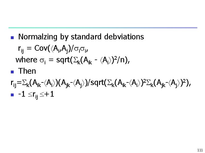
actual count – expected number k. Aik. Ajk- kikj/n = k. Aik. Ajk- (1/n) k. Aik k. Ajk, k. Aik. Ajk- n Ai Aj , k[Aik. Ajk- Ai Aj ], k(Aik - Ai )(Ajk - Aj ), where Ai is the mean of the i th raw of the adjacency matrix (1/n) k. Aik, positive: i and j has more neighbors then by chance negative: i and j has less neighbors then by chance n times covariance of two raws of the adjacency matrix Cov( Ai, Aj), n 110

Normalzing by standard debviations rij = Cov( Ai, Aj)/ i i, where i = sqrt( k(Aik - Ai )2/n), n Then rij= k(Aik- Ai )(Ajk- Aj )/sqrt( k(Aik- Ai )2 k(Ajk- Aj )2), n -1 rij +1 n 111

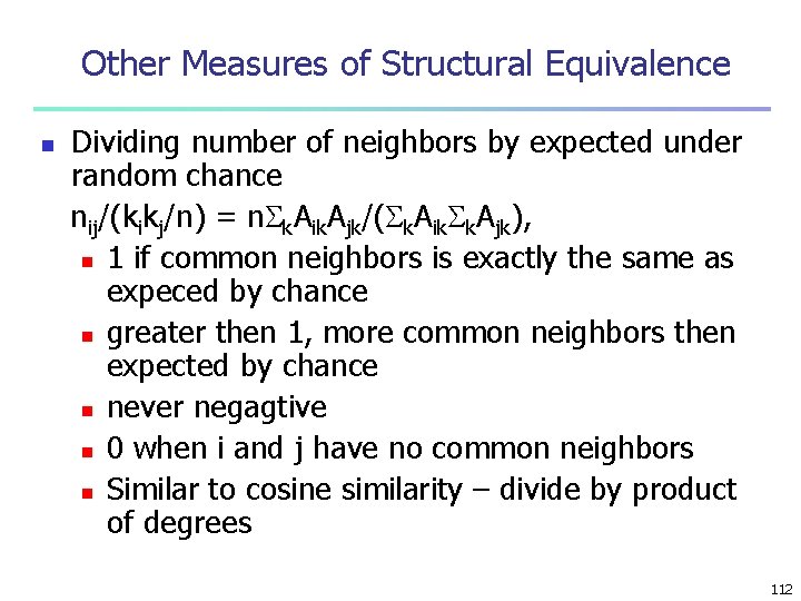
Other Measures of Structural Equivalence n Dividing number of neighbors by expected under random chance nij/(kikj/n) = n k. Aik. Ajk/( k. Aik k. Ajk), n 1 if common neighbors is exactly the same as expeced by chance n greater then 1, more common neighbors then expected by chance n never negagtive n 0 when i and j have no common neighbors n Similar to cosine similarity – divide by product of degrees 112

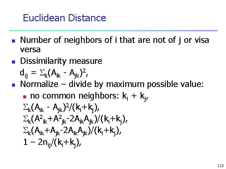
Euclidean Distance n n n Number of neighbors of i that are not of j or visa versa Dissimilarity measure dij = k(Aik - Ajk)2, Normalize – divide by maximum possible value: n no common neighbors: ki + kj, k(Aik - Ajk)2/(ki+kj), k(A 2 ik+A 2 jk-2 Aik. Ajk)/(ki+kj), k(Aik+Ajk-2 Aik. Ajk)/(ki+kj), 1 – 2 nij/(ki+kj), 113

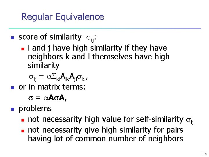
Regular Equivalence n n n score of similarity ij: n i and j have high similarity if they have neighbors k and l themselves have high similarity ij = kl. Aik. Ajl kl, or in matrix terms: = A A, problems n not necessarity high value for self-similarity ij n not necessarity give high similarity for pairs having lot of common number of neighbors 114

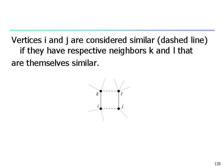
Vertices i and j are considered similar (dashed line) if they have respective neighbors k and l that are themselves similar. 115

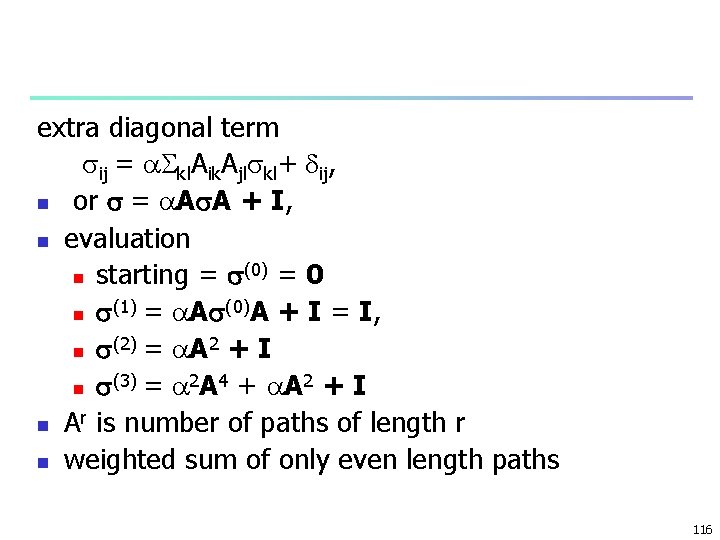
extra diagonal term ij = kl. Aik. Ajl kl+ ij, n or = A A + I, n evaluation (0) = 0 n starting = (1) = A (0)A + I = I, n (2) = A 2 + I n (3) = 2 A 4 + A 2 + I n n Ar is number of paths of length r n weighted sum of only even length paths 116

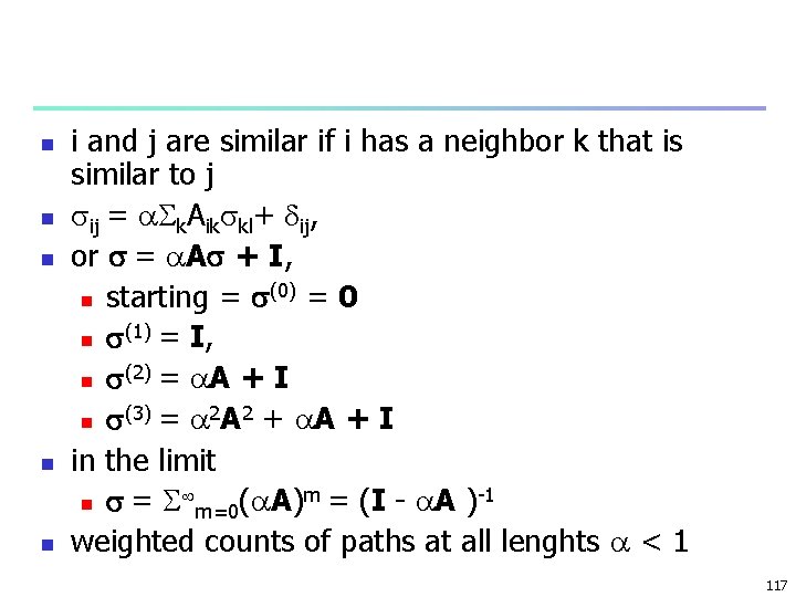
n n n i and j are similar if i has a neighbor k that is similar to j ij = k. Aik kl+ ij, or = A + I, (0) = 0 n starting = (1) = I, n (2) = A + I n (3) = 2 A 2 + A + I n in the limit m -1 n = m=0( A) = (I - A ) weighted counts of paths at all lenghts < 1 117

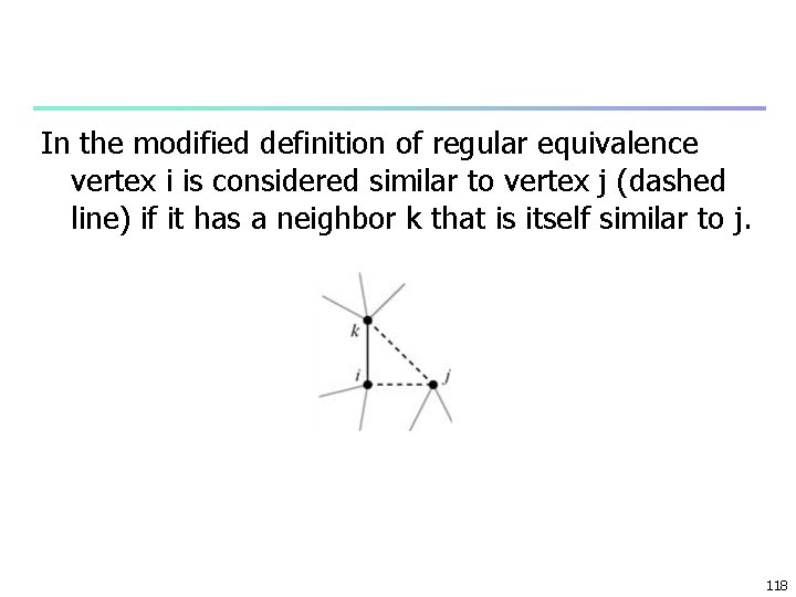
In the modified definition of regular equivalence vertex i is considered similar to vertex j (dashed line) if it has a neighbor k that is itself similar to j. 118

n n n Reminiscent of Katz cenralality Katz similarity Katz centrality of a vertex: -1 n X = (I - A ) 1, X = 1 n Sum of Katz similarities of that vertex to all others Vertices similar to others get high centrality det(I - A)=0, < 1/ 1, inverse of largest EV Generalization of structural equivalence n Common neighbors: paths of lengh 2 n Extension: weighted all paths 119

Variations Scale by degree ij = ( /ki) k. Aik kl+ ij, n or = D-1 A + I, n where Dii = ki, -1 -1 -1 n = (I - D A) = (D - A) D, n Another variation n Last term not just diagonal but includes offdiagonal elements n Non-network information is incorporated to similarity of vertex i and j. n 120

Homophily and Assortative Mixing n n n people have strong tendensy to associate with others whom they perceive as being similar to themselves disassortative mixing: associate - unlike Assortative mixing by n discrete characteristics – race, gender, nationality n scalr characteristics – age, income 121

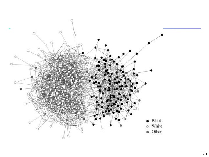
Figure 7. 10 of N-N Friendship network at a US high school. The vertices in this network represent 470 students at a US high school (ages 14 to 18 years). The vertices are color coded by race as indicated in the key. 122

123

Assortative Mixing by Categorical Variables n n significant fraction of the edges run between similar classes. n quantify – measure that fraction n tends to be 1 for a single class network A better measure: n fraction of edges between vertices of the same type minus n fraction of same type of edges if connections are random 124

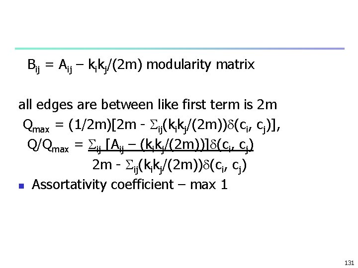
n n ci class or type i, i =1, . . . , nc number of edges between classes of the same type edge(i, j) (ci, cj) = (1/2) ij. Aij (ci, cj), n (m, n) is the Kronicer delta expeced number of edges between vertices if connections are at random: (1/2) ij[kikj/(2 m)] (ci, cj), (1/2) ij. Aij (ci, cj) - (1/2) ij[kikj/(2 m)] (ci, cj) (1/2) ij [Aij – (kikj/(2 m))] (ci, cj) 125

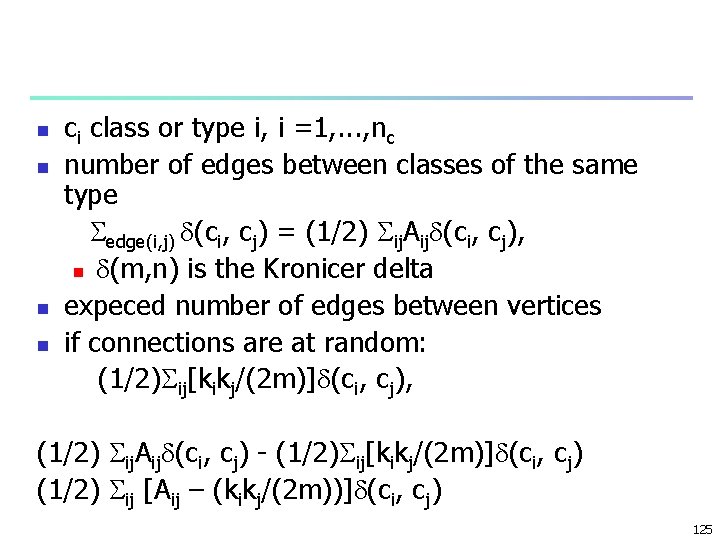
dividing by m Q = (1/2 m) ij [Aij – (kikj/(2 m))] (ci, cj), n Modularity n Extend to which like is connected to like n at most 1 n +, more edges between like than expeced by change n -, less edges between like than expeced by change – disassortative mixing n 126

Example n n n E. g. : Fig. 7. 10, types - three ethnic classifications “black, ” “white, ” “other, ” Q = 0. 305, indicating (positive) assortative mixing by race Negative values of the modularity indicate disassortative mixing. 127

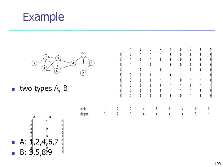
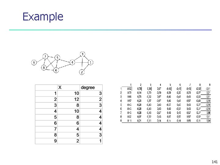
Example n n n two types A, B A: 1, 2, 4, 6, 7 B: 3, 5, 8. 9 128

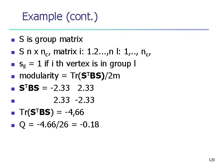
Example (cont. ) n n n n S is group matrix S n x nc, matrix i: 1. 2. . . , n l: 1, . . , nc, sil = 1 if i th vertex is in group l modularity = Tr(STBS)/2 m STBS = -2. 33 -2. 33 Tr(STBS) = -4, 66 Q = -4. 66/26 = -0. 18 129

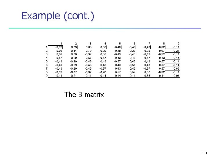
Example (cont. ) The B matrix 130

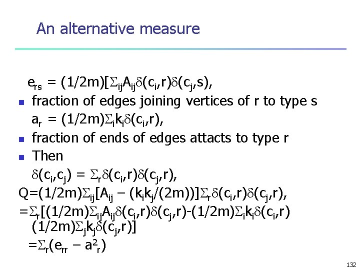
Bij = Aij – kikj/(2 m) modularity matrix all edges are between like first term is 2 m Qmax = (1/2 m)[2 m - ij(kikj/(2 m)) (ci, cj)], Q/Qmax = ij [Aij – (kikj/(2 m))] (ci, cj) 2 m - ij(kikj/(2 m)) (ci, cj) n Assortativity coefficient – max 1 131

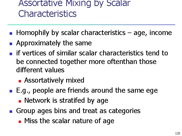
An alternative measure ers = (1/2 m)[ ij. Aij (ci, r) (cj, s), n fraction of edges joining vertices of r to type s ar = (1/2 m) iki (ci, r), n fraction of ends of edges attacts to type r n Then (ci, cj) = r (ci, r) (cj, r), Q=(1/2 m) ij[Aij – (kikj/(2 m))] r (ci, r) (cj, r), = r[(1/2 m) ij. Aij (ci, r) (cj, r)-(1/2 m) iki (ci, r) (1/2 m) jkj (cj, r)] = r(err – a 2 r) 132

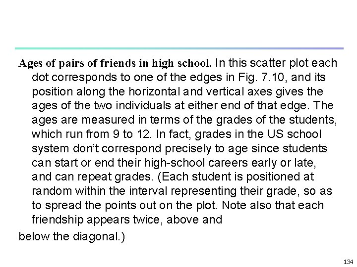
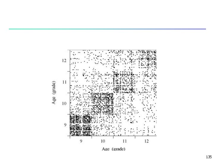
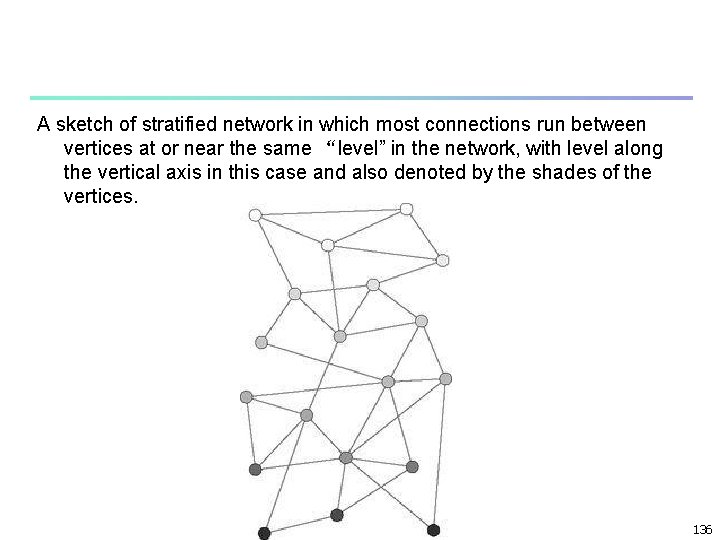
Assortative Mixing by Scalar Characteristics n n n Homophily by scalar characteristics – age, income Approximately the same if vertices of similar scalar characteristics tend to be connected together more oftenthan those different values n Assortatively mixed E. g. , people are friends around the same ege n Network is stratifed by age Group ages bins and treat as categories n Miss the scalar nature of age 133

Ages of pairs of friends in high school. In this scatter plot each dot corresponds to one of the edges in Fig. 7. 10, and its position along the horizontal and vertical axes gives the ages of the two individuals at either end of that edge. The ages are measured in terms of the grades of the students, which run from 9 to 12. In fact, grades in the US school system don’t correspond precisely to age since students can start or end their high-school careers early or late, and can repeat grades. (Each student is positioned at random within the interval representing their grade, so as to spread the points out on the plot. Note also that each friendship appears twice, above and below the diagonal. ) 134

135

A sketch of stratified network in which most connections run between vertices at or near the same “level” in the network, with level along the vertical axis in this case and also denoted by the shades of the vertices. 136

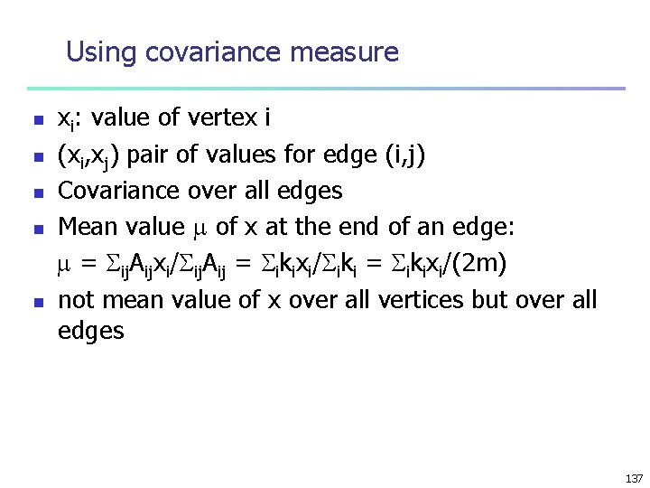
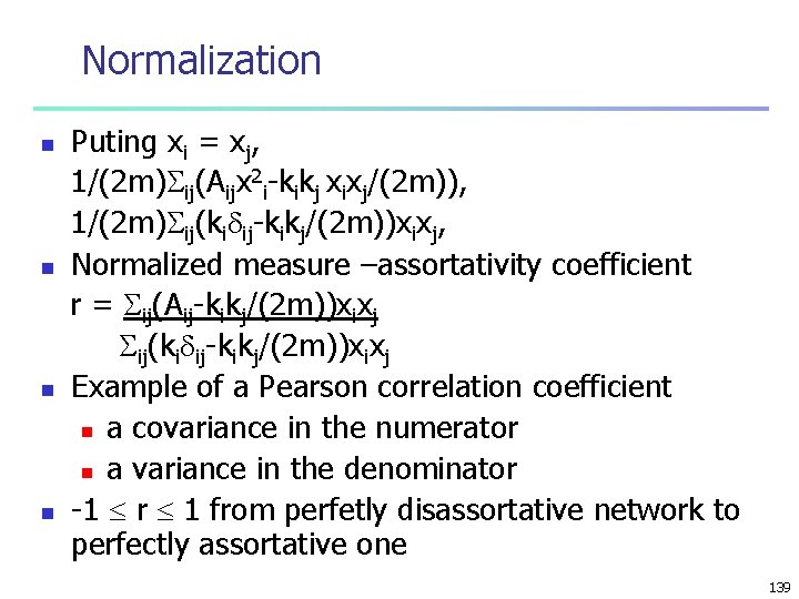
Using covariance measure n n n xi: value of vertex i (xi, xj) pair of values for edge (i, j) Covariance over all edges Mean value of x at the end of an edge: = ij. Aijxi/ ij. Aij = ikixi/ iki = ikixi/(2 m) not mean value of x over all vertices but over all edges 137

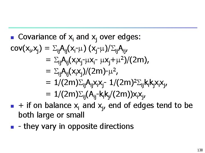
Covariance of xi and xj over edges: cov(xi, xj) = ij. Aij(xi- ) (xj- )/ ij. Aij, = ij. Aij(xixj- xi- xj+ 2)/(2 m), = ij. Aij(xixj)/(2 m)- 2, = 1/(2 m) ij. Aijxixj- 1/(2 m)2 ijkikjxixj, = 1/(2 m) ij(Aij-kikj/(2 m))xixj, n + if on balance xi and xj, end of edges tend to be both large or small n - they vary in opposite directions n 138

Normalization n n Puting xi = xj, 1/(2 m) ij(Aijx 2 i-kikj xixj/(2 m)), 1/(2 m) ij(ki ij-kikj/(2 m))xixj, Normalized measure –assortativity coefficient r = ij(Aij-kikj/(2 m))xixj ij(ki ij-kikj/(2 m))xixj Example of a Pearson correlation coefficient n a covariance in the numerator n a variance in the denominator -1 r 1 from perfetly disassortative network to perfectly assortative one 139

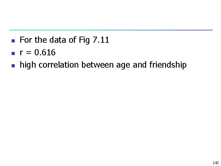
n n n For the data of Fig 7. 11 r = 0. 616 high correlation between age and friendship 140

Example 141

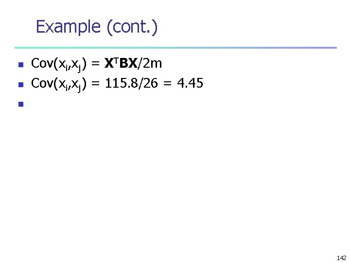
Example (cont. ) n n Cov(xi, xj) = XTBX/2 m Cov(xi, xj) = 115. 8/26 = 4. 45 n 142

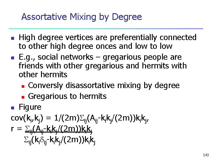
Assortative Mixing by Degree High degree vertices are preferentially connected to other high degree onces and low to low n E. g. , social networks – gregarious people are friends with other gregarious and hermits with other hermits n Conversly disassortative mixing by degree n Gregarious to hermits n Figure cov(ki, kj) = 1/(2 m) ij(Aij-kikj/(2 m))kikj, r = ij(Aij-kikj/(2 m))kikj ij(ki ij-kikj/(2 m))kikj n 143

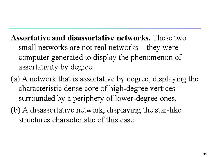
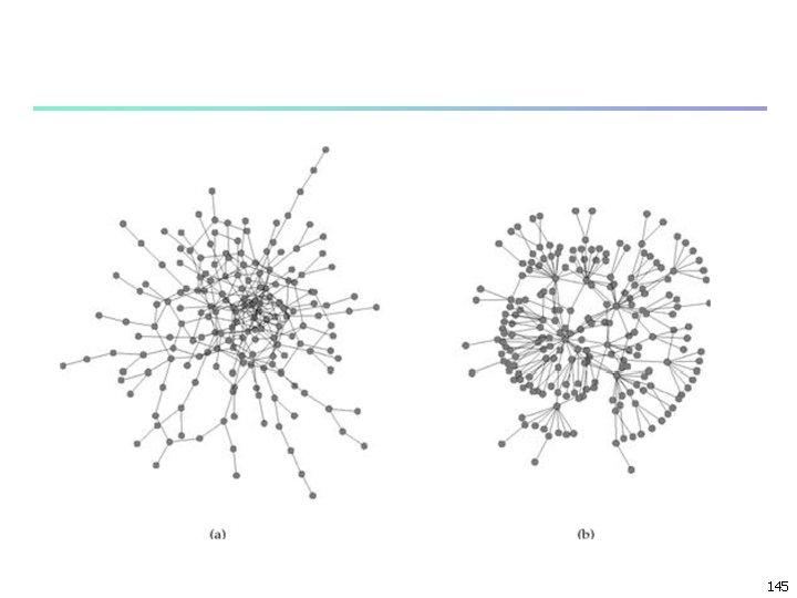
Assortative and disassortative networks. These two small networks are not real networks—they were computer generated to display the phenomenon of assortativity by degree. (a) A network that is assortative by degree, displaying the characteristic dense core of high-degree vertices surrounded by a periphery of lower-degree ones. (b) A disassortative network, displaying the star-like structures characteristic of this case. 144

145

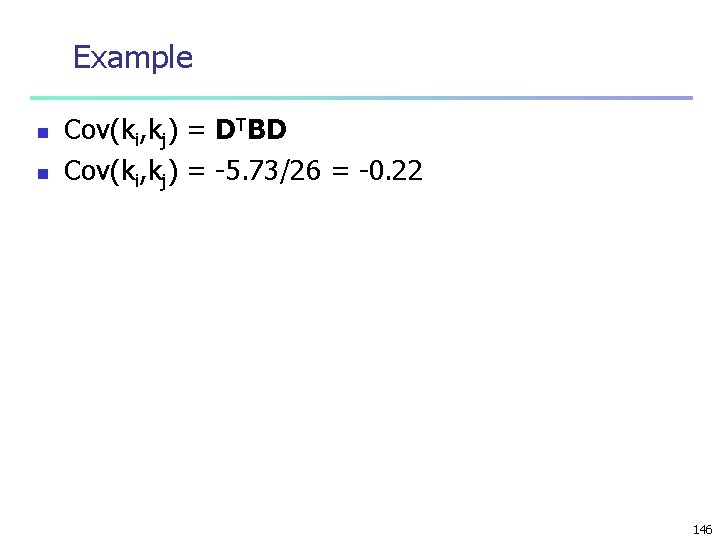
Example n n Cov(ki, kj) = DTBD Cov(ki, kj) = -5. 73/26 = -0. 22 146