MIS 644 Social Newtork Analysis 20172018 Spring Chapter

MIS 644 Social Newtork Analysis 2017/2018 Spring Chapter 6 -B Models of Network Formation 1

Outline n Introduction n Preferential Attachment n Vertex Copying Models n Network Optimization Models 2

Introduction n RNM in Chapter 6 I – structural features n giant and small components, DD, average path length modeling processes on networks n network resilience, spread of information or disieases on contact networks parameters are fixed externally n n: # vertices, m: # of edges , DD 3

Example n n n DD – power law generate a network with a DD of power law investigate its structural characteristics n analytically or computationally But no explanation why the network should have a power-law DD Different kind of models: n offer such an explanation

Generative Network Models n n Generative network models: n model mechanisms by which networks are created n hypothesized generative mechanisms n what structure they produce? Compre structure generated with the obsereved real network’s structure n suggestion – not a proof n similar mechanisms at work in the real networks

Example Models n n preferential attachment – generate power law DD generaliztions of PA vertex copying models based on optimization

Outline n Introduction n Preferential Attachment n Vertex Copying Models n Network Optimization Models 7

Preferential Attachments n n n many real networks DD approximately power-law in the tail n E. g. : Internet, www, citation and some social networks emprical data - power-law – interesting underlying processes Price in 1970 s: a simple and elegant network formation model gives rise to a power-law DD

Price’ work n n Citation net of papers having authored an important early paper – observe a PL H. Simon’s work – economic data - wealth distributions Explanation: people already have money gain money at a rate proportional to the money how much they have rich get richer – power law distribution

Assumptions of PM n new papers apear citing existing papers directed networks - acyclical no papers disapear

n new papers apear citing existing papers n c: average # papers cited by a new paper n probability proprtional to # of citations the paper got # of citations a paper gets increases with the citations it already had n n average out degree

n n n at the beginning a paper has no citatitons pure proportinality does not work citations + a constant (a) – free citations it starts off with (a) citations another interpretation: n a certain fraction of citations goes to papers choosen uniformly at random n without regard to how many citations it currently has

n n Initial conditions n Specify the starting state n how to initialize the model n large n – not depends on intial conditions n but start with a set of papers with no citations acyclical – no loops n not suitable for wwww In degree distribution – large n n parameters c, a directed and undirected networks

n n n notation: in-degree of a vertex kini, - qi, pq(n): fraction of vertices with in-degree q, whem the netowrk contains n vertices what happens when one new vertex is added? one of the citations made by that vertex n to a vertex i qi + a n probability: average in degree: q = n-1 iqi, average out-degree: c = q

n n n expected # of new ciatations by a new paper to paper i: c x prob of ciating i there are npq(n) vertices of degree q expected # of citations to all vertices with degree q: master equation – evolution of in-degree distributions: When a new vertex is added, expeced # vertices in degree q-1 to q

expeced # vertices in degree q to q+1 n n # vertices with in-degree q after adding the (n+1)th vertex: (n+1)pq(n+1) first term in RHS: # vertices previously id q

n n n q=0 newly added vertex has degree 0 no vertex has degrees less than 0 n : asymphtotic form of in-DD notation pq = pq( )

n rearraging the second n for q >=1 n calculate pq iteratively from q 0, n p 2,

n for general q n The Gamma function: n with the propertie:

n for x > 0 iterating this n We can write: n The Euler’s Beta function n d

n n multiplying and dividing by (2+a/c) = (1+a/c) or

n q in the first argument of the upper Beta function Stirling approximation for gamma function n for large q and fixed a and c n 22

n n n exponent >= 2 if c=a = 3 relevant to emprical data Price’s model – simplifying assumptions simplified and incomplete ignoring n quality and relevance of papers n development and fashions im the field n repugtation of journal and author

Simulation of Price Model n n n n Simulating netweorks implementing rules check analytical solutions generate real examples of networks metrics of real networks n E. g. : DD, clustering coef. , path lengths parameters of the simulated netork model what are the best values of parameters leading the observed metrics

n n Statistics n observed data n simple models – linear regression n estimate pareters n make inference – form and tezt hypothesis The same methodology with simulation

A simple simulation n out-degree of vertices fixed – c selection of vertices that receive edges n as a function of their in-degrees random but not uniformly

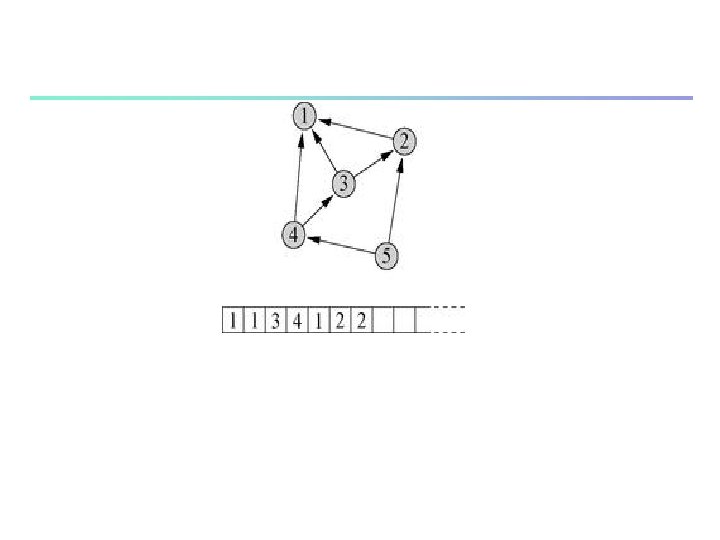
Fast way of simulating the Price Model n n i: probability of receiving an edge for node i with probability , attach the edge to a vertex proportional to its in-degree n with 1 - attach the edge to a uniformly selected vertex – 1/n total probability: n =c/(c+a) N-N pp 497 -8 n

Figure 14. 1: The vertex label list used in the simulation of Price’s model. The list (bottom) contains one entry for the target of each edge in the network (top). In this example, there are three edges that point to vertex 1 and hence there are three elements containing the number 1 in the list. Similarly there are two containing the number 2, because vertex 2 is the target of two edges. And so forth

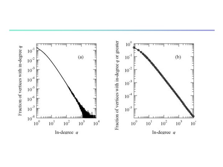
Figure 14. 2: Degree distribution in Price’s model of a growing network. (a) A histogram of the in-degree distribution for a computer-generated network with c = 3 and a = 1. 5 which was grown until it had n = 108 vertices. The simulation took about 80 seconds on the author’s computer using the fast algorithm described in the text. (b) The cumulative distribution function for the same network. The points are the results from the simulation and the solid line is the analytic solution, Eq. (14. 34)

The Model of Barabasi and Albert n n n n BA model – undirected network vertices are added one by one suitablelly choosen set of vertices connections – undirected # of connection by each vertex – c (fixed) n c being an integer connections to vertices their degree ki, vertices are only added (not removed) n no vertices with k < c, smallest degree k=c

DD of the BA Model n n n can be solved by a master equation from scrach equivalent to a special case of the Price’s model imagine – give each edge added a direction n from the vertex just added to existing that the edge connects convert into directed net – each vertex n out-degree: c n ki= qi+c, qi: in-degree as before prob ki, c+qi, Price’s model with a=c

n n n in the limit of large q The degree distribution is given by the BA model generates a degree distribution with a power-law tail always has an exponent with = 3

n n n BA model can be simulated n treting as a directed network a=c the uniform prob = ½ BA not require the offset parameter a DD without using gamma or beta furnctions never matches with real world exponents as = 3

Extensions of PA Models n n n Extensions and generalizations of PA addressing n what heppends when details of model definition are varied n more faitful to how real newtorks behave www links are added and removed any time a link can be added not just the vertex is created entire web page can disapear or apear PA process can be non-linear indegree not all vertices are equal n some pages are more interesting or imporant

Addition of extra edges n n n Price’s model bibliography no edges are added after a paper is published www is changing n links are added and removed n still has a power-law DD Simple case: edges are added but not removed generalization of BA model n vertices are added one by one n each started with c undirected edges n atached to vertex i with prob prortional to degree ki,

n n n a second process is added to the model: at each step some number w edges are added n with both ends attaching to vertices in proportion to their degree when n vertices – n(c+w) total edges w: average # of edges – can be non-integer for every new vertex added: n c+2 w new ends of edges to old vertices n two extra for each of w new extra edges

n n n prob of attachment of any one of ends of edges to any vertex i: ki/ iki, iki=2 n(c+w) pk(n): fraction of vertices with degree k when there are n vertices # of vertices of degree k, receiving a new edge when one vertex added: the master equation: k>c k =c

n taking the limit for large n, with pk = pk( ) n rearranging these equations n where B(x, y) is the Eulers beta function n since B(x, y) goes as x-y for large x

n n DD has a power law with exponent for the special case of w=0 (no additional edges are addded) n =3 BA model w > 0: exponents in the range 2 < < 3 n DD of www – directed net Generalizations of the Price’s model

Removal of edges n n n Simple case: edges can be removed at any time but added only at the initial creation of a vertex General case: adding and removing at any time removal – uniformly at random probability that any vertex i loses an edge when a single edge is removed n its two ends vanish n prob one of these ends attached to i: total # of ends attaced to i: ki, prob of i losing an edge: 2 ki/ iki,

n n n n A vertex with degree c is added then average of v edges are delated at random c – v > 0 so # of edges grow when there are n vertices: # edges: n(c-v) master eq: # of vertices with degree k increases: n whenever a vertex with degree k-1 gains an edge decreases: n when a vertex with degree k gains a new edge

n n n # vertices of degree k gaining an edge: a new process : a vertex can lose an edge: # of vertices with degree k increases: n whenever a vertex with degree k+1 loses an edge decreases: n when a vertex with degree k loses an edge # vertices of degree k losing an edge:

n vertices can have any degree k >=0 n can lose all of their edges n different form BA with k >= c master eq: k c n for k=c n

n n n can be combined where kc is Kroniker delat =1 if k=c, 0 ow exception k=0 term proportional withk-1 vanishes put p-1(n) = 0 applys for k>=0

n n n w extra edges per vertex addition c+w-v edges are added per new vertex the master equation becomes: the eq with only edge removel is a special case with w=0 assumption net # of edges added > 0, v < c+w taking the limit for large n pk = pk( )

n n n n rigth hand side contains degrees of k-1, k, k+1 not simply solve for pk in terms of pk-1, Solution using moment generating functions pk k- , exponent can take values < or > 2 v=(1/2)c+w becomes infinite DD not have power law

n n n for v < (1/2)c+w n DD power-law with a very large exponent for v > (1/2)c+w n non sensical solution with negative , Vertex removel rather then edge solution very similar with an exponent depending on the vertex lost rate n diverging as the rate of loss approaching to rate of vertex addition

Nonlinear Preferential Attachment n n n prob that a new edge attachs to a vertex is linear in the degree of the vertex reasonable at first place attachment processes might not be linear Emplrical evidence n Jeong et al – growth of several real networks n growth rate depends on network size as well They restrict observations to a relatively short periods of time measured rates plotted as a function of vertex degree

n Some networks n roughly linear preferential attachment effect n others non-linear: growth rate power of degree n n n being different then 1 they observe =0. 8 What effect would non-linear preferential attachments have on the DD of the network? n expect to see power-law behavior?

n n n n Answer: Depends on the particular fucnctional form of the attachment probablity General approach – Krapivsky et al attachment kernel ak, specifies the functional form of the attachment probability For the BA model - attachment linearly with degree - ak= k For Jeong et al - ak= k ,

n n n attachment kernel – not probability normalized probability for a new edge attached to a vertex i with degree ki: ak/ kak, Consider a growing netowrk pk(n): fraction of vertices with degree k when the network has n vertices average of c new edges are added with each new vertex preferential attachment non-linear - ak,

n when a new vertices is added expected # of vertices of degree k receiving a connection n where n the master eq: n

n n n pk-1(n): fraction of new vertices of degree k when vertices of degree k-1 gets an new edge pk(n): vertecis of degree k lost when they get new edges to become vertices of degree k+1 The only exception: vertices of degree c

n n n taking the limit as n n pk – pk( ) and - ( ) for k > c and for k=c depends on DD but independent of k rearranging 56

n n n Applying the latter repeatedly the value of ? letting n 57

n n canceling from both sides Solve and substitute into recursive form of teh master eq – not solvable in closed form for many attachment kernels Approximated But functional form of DD pk, 58

Example: n n n Jeong et a’s network attachments goes as k , <1 by Krapivsky et a’s approach: this DD not to havde a power-law tail complared to the linear attachment Power-law form is sensitive to the precise shape of the attachment kernel 59

n n After some manipuations and approximations For large k the asymptotic form of pk: for ½ < <1 distributions: streched exponential n dominant contribution to prob falls off as a exponential of power of k n 1 - < 1 – falls off more slowly than an ordinary exponential in k n faster than a power-law in a lineear PA n power-law spetial feature of BA – linear PA 60

n for =1/2 for ¼ < 1/3 and 1/5 < < ¼ Different forms are obtained Fig 4. 8 of N-N : DD for =0. 8 along with the asymptotic form Convex form in the semi-log scale - function decaying slower than an exponential 61

n Degree distribution for sublinear preferential attachment. This plot shows the fraction p of vertices with degree k in a growing network with attachment kernel kγ as described in the text. In this case γ = 0. 8 and c = 3. The points are results from computer simulations, averaged over 100 networks of (final) size 107 vertices each. The solid line is the exact solution, Eq. (14. 112), evaluated numerically. The dashed line is the asymptotic form, Eq. (14. 119), with the overall constant of proportionality chosen to coincide with the exact solution for large values of k k γ 62

Fig 14. 8 of N-N 63

n n n calculate the DD for superlinear PA , i. e. , for > 1. shows some interesting behaviors: for one vertex to emerge as a “leader” in the network, gaining a non-zero fraction of all edges, with the rest of the vertices having small degree (almost all having degree less than some fixed constant) 64

Vertices of Varying Quality or Attachments n n n In BA model - assume that: all vertices of a given degree are equally likely to gain a new edge E. g. , n all papers not cited before – equally likely to get a citation n all web page no one linked equaly likely to be linked In real world: papers or websites – quality, makes importaant differences 65

n n n Variations in intrinsic quality or attractiveness of a vertices n effects on DD PL by PA might completely disappear Explains observed PL A network growth model by Bainconi and Barabasi n includes efects of varying node quality – fitness PL disappears but for a given fitness level vertices follow PL 66

Bianconi-Barabasi Model n n n Vertices are added one by one each with c undirected edges Each vertex i has a fitness i, assigned whan the vertex is created, never changed thereafter Fitnesses – real numbers drawn from some prob. distribution p( ) n prob. of a value folling between and +d is p( ) Attachment kernel ai( ) = k, The general model by Krapivsky and Rener 67

n n n The model can be solved by the same preocedures Example BB model n Attaschment kernel – linear in k and fitness n ai( ) = k, DD with a particular value of fitness PL with an exponent: However the overall DD may or may not have PL depending on p( ) 68

n n The trivial choice: n All vertices have the same n Reduces to the original BA model When broadly distributed: n DD sum of distributions with PLs n Not yield a PL 69

Outline n Introduction n Preferential Attachment n Vertex Copying Models n Network Optimization Models 70

Vertex Copying Models n n n PA models – power-law n citation nets, www PA not the only mechanism for network growth nor generating power-laws PA: new paper cites more likely – frequently cited papers anther way of thinking n researchers are copying citations from the bibliographies of papers they read

n n Klienberg et al – alternative mechanism for network formation n this idea one step further what if people simply copied the entire bibliography of a paper to create their own paper This process with sligth modifications – power-law DD Problems: n 1 - unlikley to copy the entier bibliography n 2 - if a paper not cited – cannot get a citation n a paper never cited - gets no citations

n n n Some little changes: Assume that some fraction of the entities in the bib. are copied remainder of the bib. – other papers n many ways of selecting e. g. : uniformly at random ensure problems 1 and 2 are solved Kleinberg at al – original model n more complex n for www

n n Each new vertex added – out degree c n Bibs. are of the same size choose uniformly at random a previous vertex for each entity in the bib. of this previous vertex n with prob. < 1: copy the entity to the bib. n with prob. 1 - : choose a vertex uniformly at random from the netwrok and add to the bib. c of the bib. of new paper is copied from a choosen vertex, the remainder uniformly at random inperfect copying

n n n specify starting state of the netowork asymptotic properties do not depend on But for example: n there are n 0 > c vertices – for each c pointers to others at random Solve DD: Prob. of vertex i receives an incoming edge from a new vertex n 1 -copy a bib. from a vertex already cited i n 2 -i one of the vertices choosen at random

n n n n an existing vertex has a link to i Prob. that new vertex will copy links of the verex : 1/n i has in-degree qi, the chance that any of these vertics is choosen qi/n The chance of copy: Total prob: qi/n, Average # links the new verex randomly selects: n (1 - )c, i being a target of one of them: 1/n Overall : (1 - )c/n

n Total prob that vertex i gets a link: n Define pq(n): fraction of vertices with in-degree q when there are n vertices in the network Total expected # of vertices with in-degree q n Define a new constant a by n

n n n then Same as original Price’s model Master eq the same as Price’s model For the evolution of pk, DD follows a power-low with the exponent:

n n n Exponents in the rane 2 to How faithfully vertices are copied n Faithful copies close to 1 – exponents close to 2 n Sloppy copies – large exponents VC networks not identical in every respects to PA n in VC – vertices are similar - correlated n in PA – independent – not correlated Real nets – power-law Not neccessarily PA –CV or even another mechanism 79

Outline n Introduction n Preferential Attachment n Vertex Copying Models n Network Optimization Models 80

Network Optimization Models n n network structure - by the way network grows n how newly added vertices connect to others n Random processes - decentralized An alaternative network formation mechanism n structural optimization In some cases: transportation, distribution n network specifically designed – goal(s) E. g. , n delivsry of packages n Transportation of airline passengers

n n n Structure – goal eficiently E. g. , airline networks – hub spoke arrangements n samall # of busy hub airports n large # of minor destinations Not reasonable - many flights between samall ports Passengers can reach samall port via hubs hub-spoke design of the nework n Eficiency, profitabbility n Stell passengers can travel 82