Measures of Location and Outliers Descriptive Statistics 1

Measures of Location and Outliers Descriptive Statistics 1

Summarizing Numerical Distributions � To ◦ ◦ describe a distribution we recall “SOCS” Shape (Distribution) Outliers Center Spread (Variation) � We have seen that outliers may show up visually but not always.

Measures of Location � Measures of location tell us about an observation’s relative standing in the distribution � They give us the tools to numerically identify outliers. � Common measures of location are: ◦ Percentiles ◦ Quartiles 3

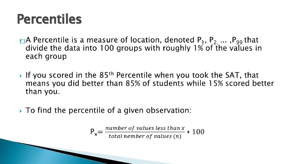
Percentiles �

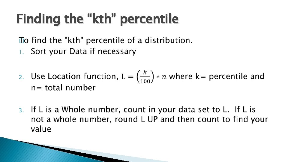
Finding the “kth” percentile �

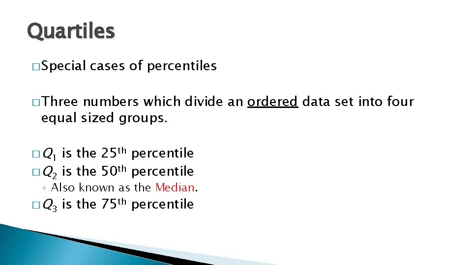
Quartiles � Special cases of percentiles � Three numbers which divide an ordered data set into four equal sized groups. � Q 1 is the 25 th percentile � Q 2 is the 50 th percentile ◦ Also known as the Median. � Q 3 is the 75 th percentile

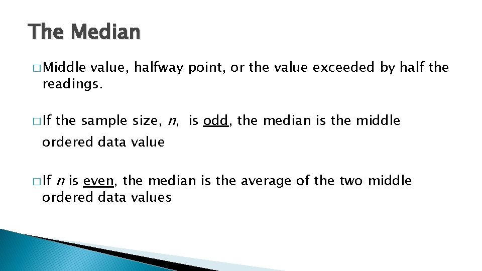
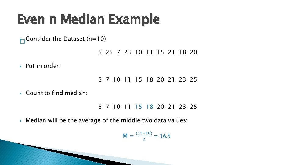
The Median � Middle value, halfway point, or the value exceeded by half the readings. � If the sample size, n, is odd, the median is the middle ordered data value � If n is even, the median is the average of the two middle ordered data values

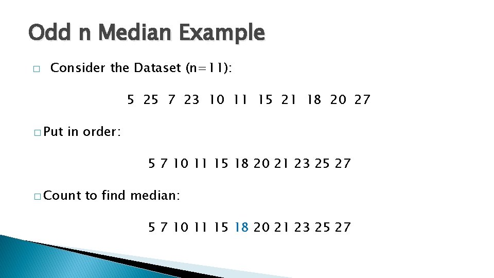
Odd n Median Example � Consider the Dataset (n=11): 5 25 7 23 10 11 15 21 18 20 27 � Put in order: 5 7 10 11 15 18 20 21 23 25 27 � Count to find median: 5 7 10 11 15 18 20 21 23 25 27

Even n Median Example �

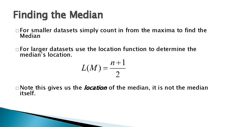
Finding the Median � For smaller datasets simply count in from the maxima to find the Median � For larger datasets use the location function to determine the median’s location. this gives us the location of the median, it is not the median itself. � Note

Finding the Quartiles � Order the data and find the median. � For Q 1, look at the lower half of the data values, those to the left of the median location; find the median of the lower half. � For Q 3, look at the upper half of the data values, those to the right of the median location; find the median of the upper half.

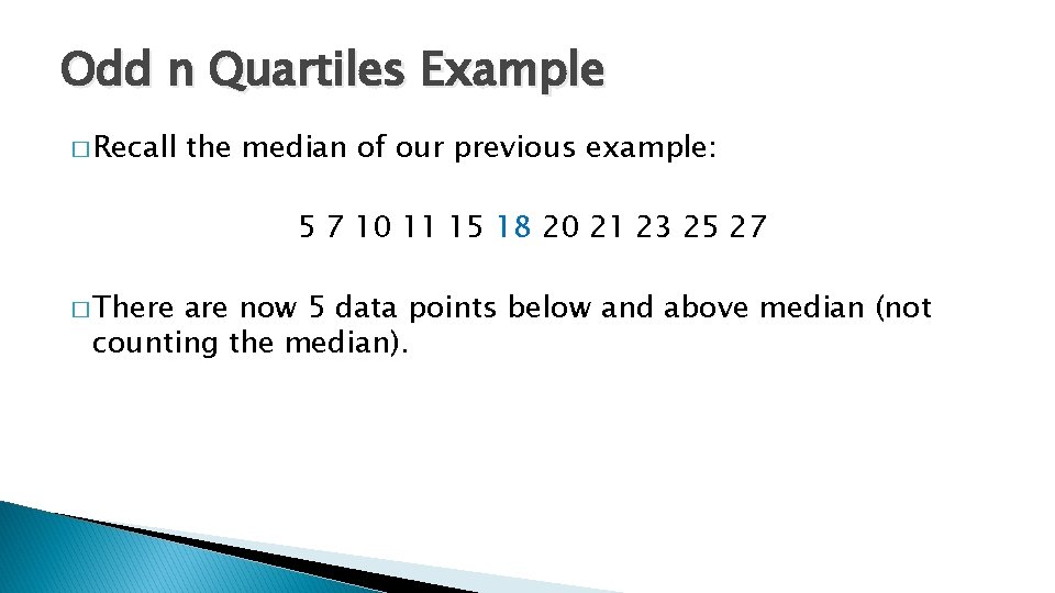
Odd n Quartiles Example � Recall the median of our previous example: 5 7 10 11 15 18 20 21 23 25 27 � There are now 5 data points below and above median (not counting the median).

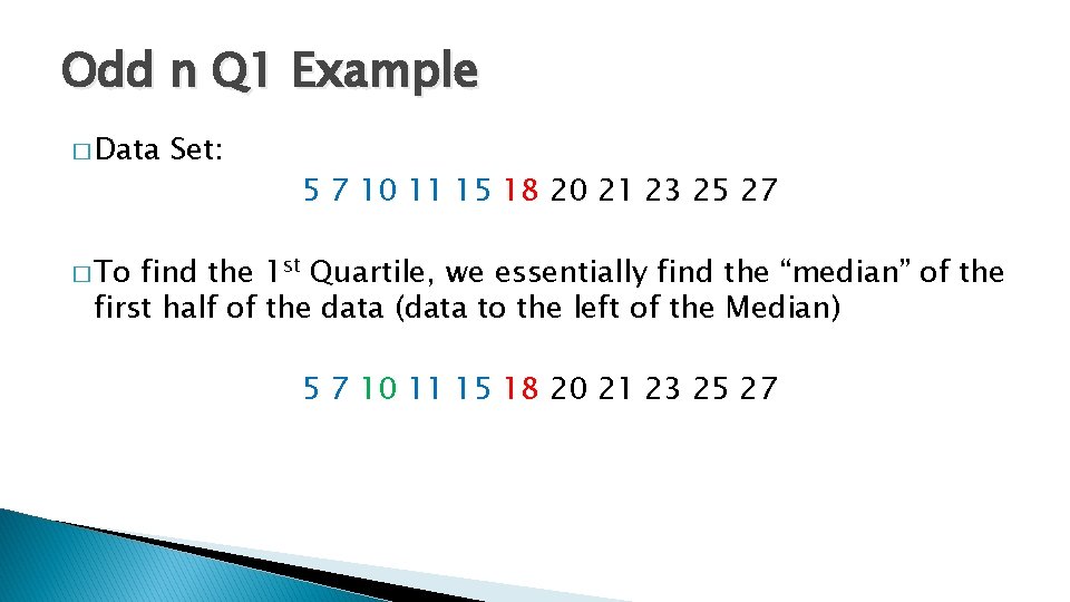
Odd n Q 1 Example � Data Set: 5 7 10 11 15 18 20 21 23 25 27 � To find the 1 st Quartile, we essentially find the “median” of the first half of the data (data to the left of the Median) 5 7 10 11 15 18 20 21 23 25 27

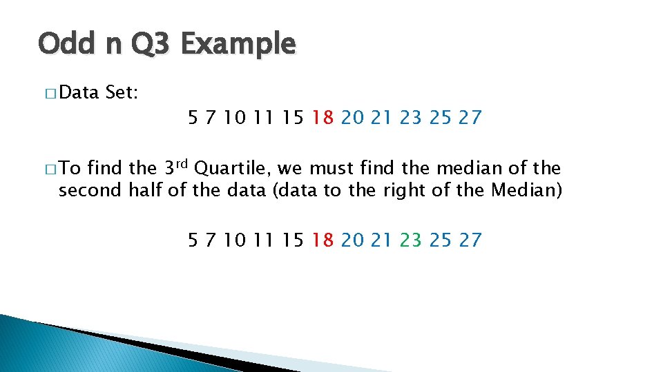
Odd n Q 3 Example � Data Set: 5 7 10 11 15 18 20 21 23 25 27 � To find the 3 rd Quartile, we must find the median of the second half of the data (data to the right of the Median) 5 7 10 11 15 18 20 21 23 25 27

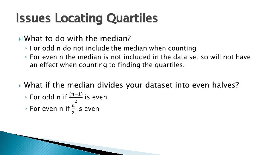
Issues Locating Quartiles �

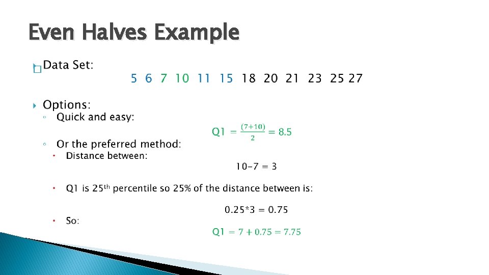
Even Halves Example �

Interquartile Range interquartile range (IQR) is the difference between the third and first quartiles. � The IQR = Q 3 – Q 1 � The IQR is measure of spread that only takes into account the middle 50% of the data

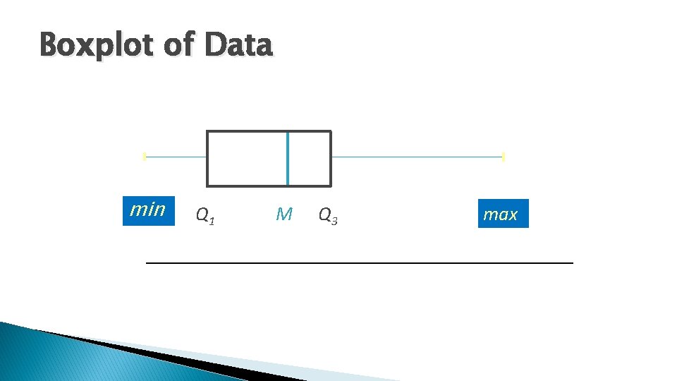
Five Number Summary � This simple summary displays the distribution of the data using specific values. Minimum Q 1 Median Q 3 Maximum �A boxplot is a graphical representation of the five-number summary

Boxplot � Central �A box spans Q 1 and Q 3. line in the box marks the median M. � Lines (or whiskers) extend from the box out to the minimum and maximum when there are no outliers in the data set. � If outliers are present, the whiskers will often only extend to the next highest or lowest value in the data set.

Boxplot of Data min Q 1 M Q 3 max

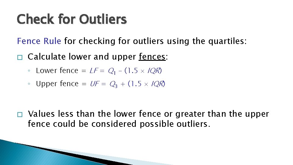
Check for Outliers Fence Rule for checking for outliers using the quartiles: � Calculate lower and upper fences: ◦ Lower fence = LF = Q 1 – (1. 5 IQR) ◦ Upper fence = UF = Q 3 + (1. 5 IQR) � Values less than the lower fence or greater than the upper fence could be considered possible outliers.

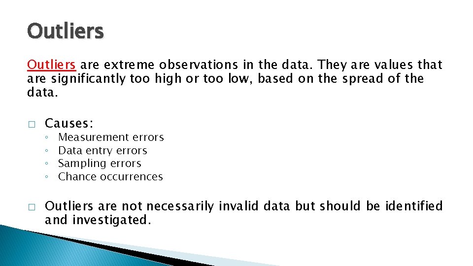
Outliers are extreme observations in the data. They are values that are significantly too high or too low, based on the spread of the data. � Causes: ◦ ◦ � Measurement errors Data entry errors Sampling errors Chance occurrences Outliers are not necessarily invalid data but should be identified and investigated.

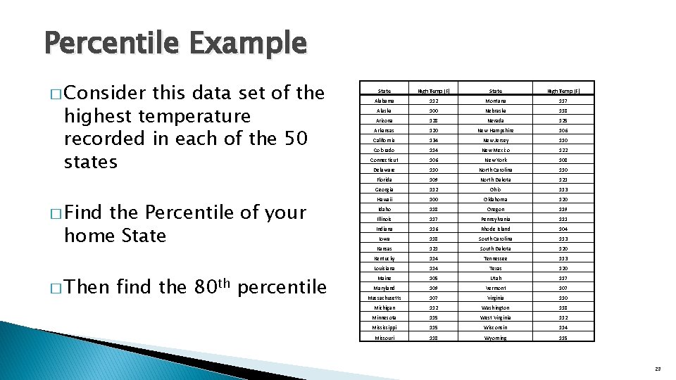
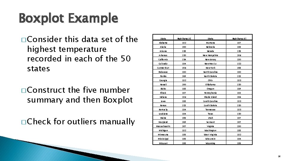
Percentile Example � Consider this data set of the highest temperature recorded in each of the 50 states � Find the Percentile of your home State � Then find the 80 th percentile State High Temp (F) Alabama 112 Montana 117 Alaska 100 Nebraska 118 Arizona 128 Nevada 125 Arkansas 120 New Hampshire 106 California 134 New Jersey 110 Colorado 114 New Mexico 122 Connecticut 106 New York 108 Delaware 110 North Carolina 110 Florida 109 North Dakota 121 Georgia 112 Ohio 113 Hawaii 100 Oklahoma 120 Idaho 118 Oregon 119 Illinois 117 Pennsylvania 111 Indiana 116 Rhode Island 104 Iowa 118 South Carolina 113 Kansas 121 South Dakota 120 Kentucky 114 Tennessee 113 Louisiana 114 Texas 120 Maine 105 Utah 117 Maryland 109 Vermont 107 Massachusetts 107 Virginia 110 Michigan 112 Washington 118 Minnesota 115 West Virginia 112 Mississippi 115 Wisconsin 114 Missouri 118 Wyoming 115 23

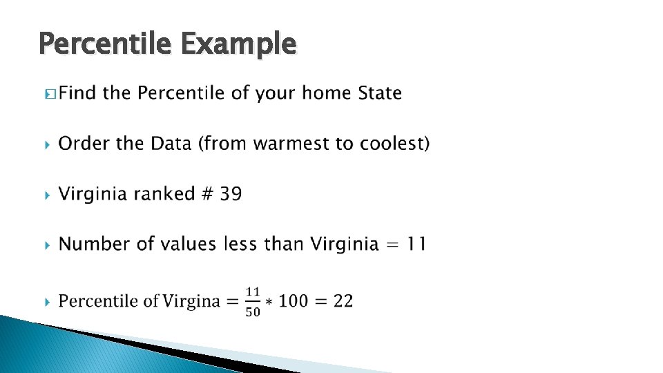
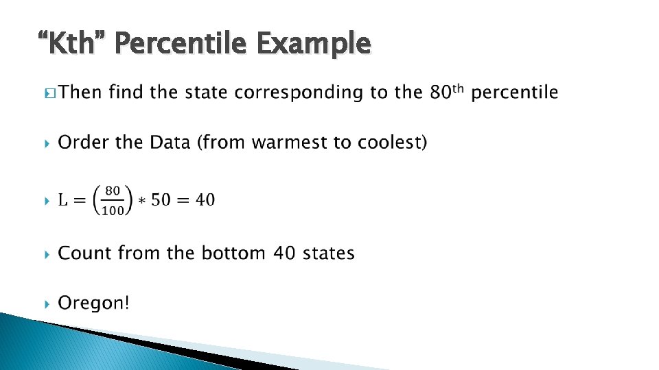
Percentile Example �

“Kth” Percentile Example �

Boxplot Example � Consider this data set of the highest temperature recorded in each of the 50 states � Construct the five number summary and then Boxplot � Check for outliers manually State High Temp (F) Alabama 112 Montana 117 Alaska 100 Nebraska 118 Arizona 128 Nevada 125 Arkansas 120 New Hampshire 106 California 134 New Jersey 110 Colorado 114 New Mexico 122 Connecticut 106 New York 108 Delaware 110 North Carolina 110 Florida 109 North Dakota 121 Georgia 112 Ohio 113 Hawaii 100 Oklahoma 120 Idaho 118 Oregon 119 Illinois 117 Pennsylvania 111 Indiana 116 Rhode Island 104 Iowa 118 South Carolina 113 Kansas 121 South Dakota 120 Kentucky 114 Tennessee 113 Louisiana 114 Texas 120 Maine 105 Utah 117 Maryland 109 Vermont 107 Massachusetts 107 Virginia 110 Michigan 112 Washington 118 Minnesota 115 West Virginia 112 Mississippi 115 Wisconsin 114 Missouri 118 Wyoming 115 26

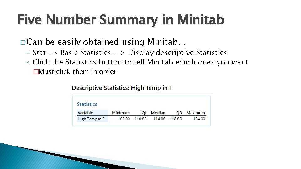
Five Number Summary in Minitab � Can be easily obtained using Minitab… ◦ Stat -> Basic Statistics - > Display descriptive Statistics ◦ Click the Statistics button to tell Minitab which ones you want �Must click them in order

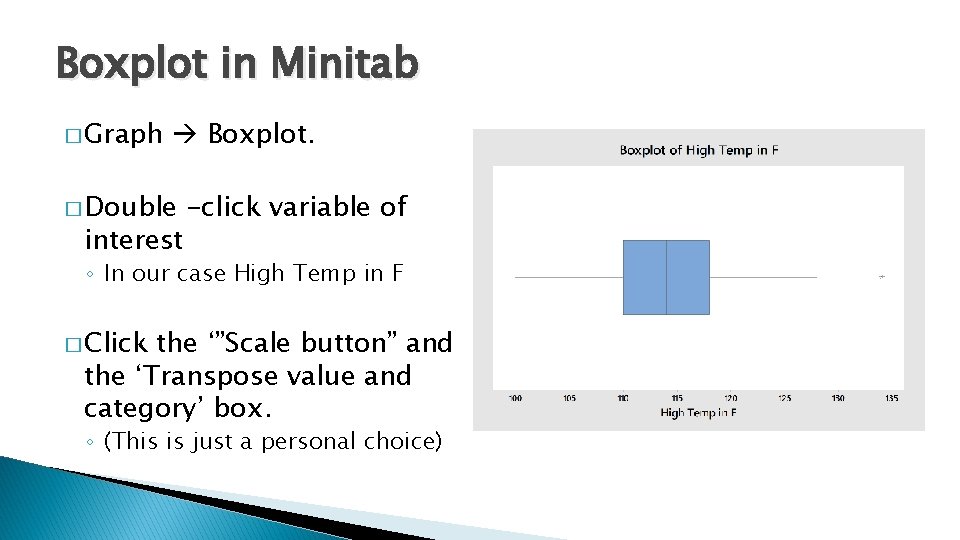
Boxplot in Minitab � Graph Boxplot. � Double interest -click variable of ◦ In our case High Temp in F � Click the ‘”Scale button” and the ‘Transpose value and category’ box. ◦ (This is just a personal choice)

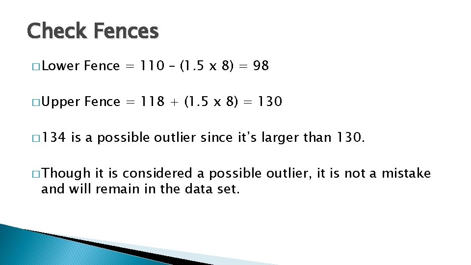
Check Fences � Lower Fence = 110 – (1. 5 x 8) = 98 � Upper Fence = 118 + (1. 5 x 8) = 130 � 134 is a possible outlier since it’s larger than 130. � Though it is considered a possible outlier, it is not a mistake and will remain in the data set.