LECTURE 02 Descriptive Statistics MGT 601 Descriptive Statistics

LECTURE 02 Descriptive Statistics MGT 601

Descriptive Statistics Table 1: Wages of 120 workers in Dollars 67 45 56 58 57 61 65 60 60 67 63 57 50 56 58 86 81 60 60 68 57 64 74 56 59 64 82 72 65 69 85 68 74 57 58 91 76 72 65 68 67 67 67 60 58 64 77 79 66 73 60 86 77 60 61 64 81 70 65 68 75 63 61 63 62 61 76 70 73 74 55 60 85 64 91 62 66 58 73 68 67 98 66 85 74 69 62 78 71 67 68 83 66 80 72 57 63 58 73 76 51 76 60 75 57 81 62 71 66 52 54 70 61 75 73 66 63 76 73 79

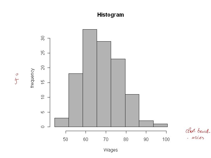
Frequency distribution Wages No of workers 45 -51 52 -58 59 -65 66 -72 73 -79 80 -86 87 -93 94 -100 Total 3 18 33 29 23 11 2 1 120

Frequency distribution Class Boundaries f Relative frequency Cumulative frequency Midpoints (X) 44. 5 -51. 5 -58. 5 -65. 5 -72. 5 -79. 5 -86. 5 -93. 5 -100. 5 Total 3 18 33 29 23 11 2 1 120 0. 025 0. 150 0. 275 0. 242 0. 191 0. 092 0. 017 0. 008 3 3+18=21 21+33=54 54+29=83 83+23=106 106+11=117 117+2=119 119+1=120 48 55 62 69 76 83 90 97

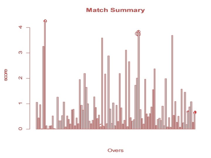
Graphical Presentation of Data One of the important functions of Statistics is to present complex and unorganized (raw) data in such a manner that it would easily be understandable at a glance. This is often best accomplished by presenting the data in a pictorial (or graphical) form. • Types of Graphs 1. Histogram 2. Frequency polygon 3. Frequency curve 4. Cumulative frequency polygon (Ogive) • We will use the frequency distribution (table) for presenting these graphs.

Frequency Polygon

Cumulative Frequency Polygon (Ogive)

Measures of Central Tendency • Introduction For practical purposes the condensation of data set into a frequency distribution and the visual presentation are not enough. Particularly, when two or more different data sets are to be compared. • A data set can be summarized in a single value. Such a value, usually somewhere in the center and representing the entire data set, is a value at which the data have the tendency to concentrate. The tendency of the observations to cluster in the central part of the data set is called Central Tendency and the methods of computing this central value are called Measures of Central Tendency. • Main measures of Central Tendency or Averages 1. Arithmetic Mean 2. Median 3. Mode

Mean=67. 658 Class limits 45 -51 52 -58 59 -65 66 -72 73 -79 80 -86 87 -93 94 -100 Total f Mid-Points 3 18 33 29 23 11 2 1 120 48 55 62 69 76 83 90 97 (X) f. X 144 990 2046 2001 1748 913 180 97 8119

Median=66. 948 Class Boundaries f Cumulative frequency 44. 5 -51. 5 -58. 5 -65. 5 -72. 5 -79. 5 -86. 5 -93. 5 -100. 5 Total 3 18 33 29 23 11 2 1 120 3 3+18=21 21+33=54 54+29=83 83+23=106 106+11=117 117+2=119 119+1=120

Mode=64. 026 Class Boundaries f 44. 5 -51. 5 -58. 5 -65. 5 -72. 5 -79. 5 -86. 5 -93. 5 -100. 5 3 18 33 29 23 11 2 1

Measures of Dispersion • Introduction • It is quite possible that two or more data sets may have the same average (mean, median, mode) but their individual observations may differ considerably from the average. Thus a value of central tendency does not adequately describe the data. We therefore need some additional information concerning how the data are dispersed about the average. This is done by measuring the dispersion by which we mean the extent to which the observations in a sample or in a population vary about their mean. A quantity that measures this characteristic, is called a measure of dispersion, scatter, or variability.

Main Measures of Dispersion i) Range ii) Quartile Deviation. iii)Mean Deviation. iv)Standard Deviation/Variance.

Standard Deviation Class limits f X 45 -51 52 -58 59 -65 66 -72 73 -79 80 -86 87 -93 94 -100 Total 3 18 33 29 23 11 2 1 120 48 55 62 69 76 83 90 97 -19. 658 -12. 658 -5. 658 1. 342 8. 342 15. 342 22. 342 29. 342

Statistical Package for the Social Sciences - (SPSS) • Originally it is an acronym of Statistical Package for the Social Science but now it stands for Statistical Product and Service Solutions • One of the most popular statistical packages which can perform highly complex data manipulation and analysis with simple instructions

Opening SPSS • The default window will have the data editor • There are two sheets in the window: 1. Data view 2. Variable view

Data View window • The Data View window This window shows the actual data values and the name of the variables. • Click on the tab labeled Variable View Click

Variable view window • Name – The first character of the variable name must be alphabetic – Variable names must be unique, and have to be less than 64 characters. – Spaces are NOT allowed.

Variable View window: Type • Type – Click on the ‘type’ box. The two basic types of variables that you will use are numeric and string. This column enables you to specify the type of variable.

Variable View window: Width • Width – Width allows you to determine the number of characters SPSS will allow to be entered for the variable

Variable View window: Decimals • Decimals – Number of decimals – It has to be less than or equal to 16

Variable View window: Label • Label – You can specify the details of the variable – You can write characters with spaces up to 256 characters

Variable View window: Values • Values – This is used and to suggest which numbers represent which categories when the variable represents a category

Defining the value labels • Click the cell in the values column as shown below • For the value, and the label, you can put up to 60 characters. • After defining the values click add and then click OK. Click

Practice 1 • How would you put the following information into SPSS? Value = 1 represents Male and Value = 2 represents Female

Practice 1 (Solution Sample) Click

Click

Saving the data • To save the data file you created simply click ‘file’ and click ‘save as. ’ You can save the file in different forms by clicking “Save as type. ” Click