Stat 112 Notes 15 Today Outliers and influential

Stat 112 Notes 15 • Today: – Outliers and influential points. • Homework 4 due on Thursday.

Outliers and Influential Observations in Simple Regression • Outlier: Any really unusual observation. • Outlier in the X direction (called high leverage point): Has the potential to influence the regression line. • Outlier in the direction of the scatterplot (outliers in residuals): An observation that deviates from the overall pattern of relationship between Y and X. Residual is large in absolute value. • Influential observation: Point that if it is removed would markedly change the statistical analysis. For simple linear regression, points that are outliers in the x direction are often influential.

Housing Prices and Crime Rates • A community in the Philadelphia area is interested in how crime rates are associated with property values. If low crime rates increase property values, the community might be able to cover the costs of increased police protection by gains in tax revenues from higher property values. • The town council looked at a recent issue of Philadelphia Magazine (April 1996) and found data for itself and 109 other communities in Pennsylvania near Philadelphia. Data is in philacrimerate. JMP. House price = Average house price for sales during most recent year, Crime Rate=Rate of crimes per 1000 population.

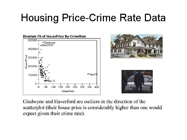
Housing Price-Crime Rate Data

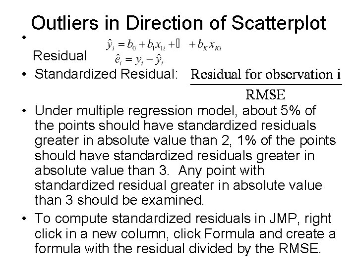
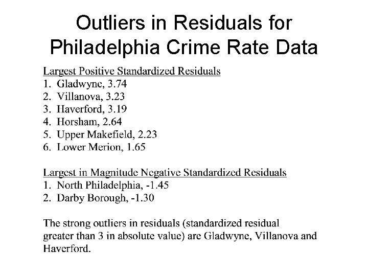
• Outliers in Direction of Scatterplot Residual • Standardized Residual: • Under multiple regression model, about 5% of the points should have standardized residuals greater in absolute value than 2, 1% of the points should have standardized residuals greater in absolute value than 3. Any point with standardized residual greater in absolute value than 3 should be examined. • To compute standardized residuals in JMP, right click in a new column, click Formula and create a formula with the residual divided by the RMSE.

Outliers in Residuals for Philadelphia Crime Rate Data

Influential Points and Leverage Points • Influential observation: Point that if it is removed would markedly change the statistical analysis. For simple linear regression, points that are outliers in the X direction are often influential. • Leverage point: Point that is an outlier in the X direction that has the potential to be influential. It will be influential if its residual is of moderately large magnitude.

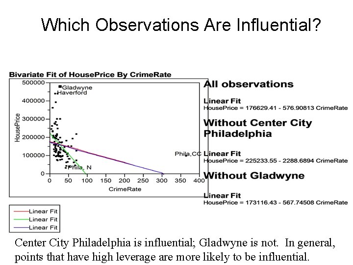
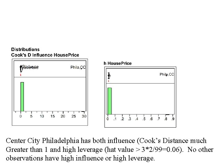
Which Observations Are Influential? Center City Philadelphia is influential; Gladwyne is not. In general, points that have high leverage are more likely to be influential.

Excluding Observations from Analysis in JMP • To exclude an observation from the regression analysis in JMP, go to the row of the observation, click Rows and then click Exclude/Unexclude. A red circle with a diagonal line through it should appear next to the observation. • To put the observation back into the analysis, go to the row of the observation, click Rows and then click Exclude/Unexclude. The red circle should no longer appear next to the observation.

Formal measures of leverage and influence • Leverage: “Hat values” (JMP calls them hats) • Influence: Cook’s Distance (JMP calls them Cook’s D Influence). • To obtain them in JMP, click Analyze, Fit Model, put Y variable in Y and X variable in Model Effects box. Click Run Model box. After model is fit, click red triangle next to Response. Click Save Columns and then Click Hats for Leverages and Click Cook’s D Influences for Cook’s Distances. • To sort observations in terms of Cook’s Distance or Leverage, click Tables, Sort and then put variable you want to sort by in By box.

Center City Philadelphia has both influence (Cook’s Distance much Greater than 1 and high leverage (hat value > 3*2/99=0. 06). No other observations have high influence or high leverage.

Rules of Thumb for High Leverage and High Influence • High Leverage Any observation with a leverage (hat value) > (3 * # of coefficients in regression model)/n has high leverage, where # of coefficients in regression model = 2 for simple linear regression. n=number of observations. • High Influence: Any observation with a Cook’s Distance greater than 1 indicates a high influence.

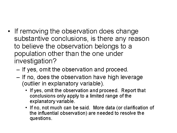
What to Do About Suspected Influential Observations? Does removing the observation change the substantive conclusions? • If not, can say something like “Observation x has high influence relative to all other observations but we tried refitting the regression without Observation x and our main conclusions didn’t change. ”

• If removing the observation does change substantive conclusions, is there any reason to believe the observation belongs to a population other than the one under investigation? – If yes, omit the observation and proceed. – If no, does the observation have high leverage (outlier in explanatory variable). • If yes, omit the observation and proceed. Report that conclusions only apply to a limited range of the explanatory variable. • If no, not much can be said. More data (or clarification of the influential observation) are needed to resolve the questions.

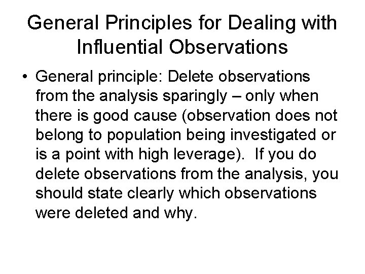
General Principles for Dealing with Influential Observations • General principle: Delete observations from the analysis sparingly – only when there is good cause (observation does not belong to population being investigated or is a point with high leverage). If you do delete observations from the analysis, you should state clearly which observations were deleted and why.

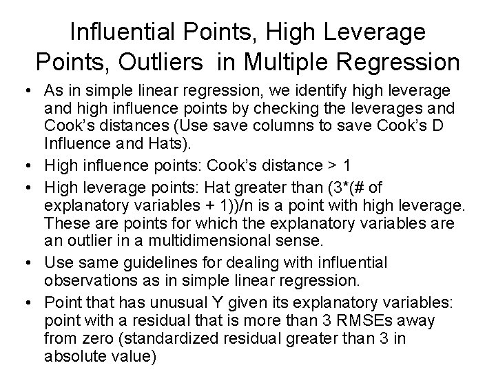
Influential Points, High Leverage Points, Outliers in Multiple Regression • As in simple linear regression, we identify high leverage and high influence points by checking the leverages and Cook’s distances (Use save columns to save Cook’s D Influence and Hats). • High influence points: Cook’s distance > 1 • High leverage points: Hat greater than (3*(# of explanatory variables + 1))/n is a point with high leverage. These are points for which the explanatory variables are an outlier in a multidimensional sense. • Use same guidelines for dealing with influential observations as in simple linear regression. • Point that has unusual Y given its explanatory variables: point with a residual that is more than 3 RMSEs away from zero (standardized residual greater than 3 in absolute value)

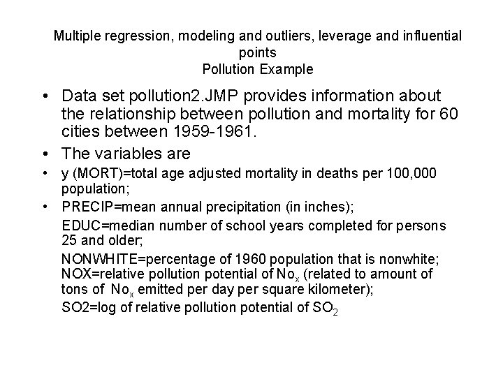
Multiple regression, modeling and outliers, leverage and influential points Pollution Example • Data set pollution 2. JMP provides information about the relationship between pollution and mortality for 60 cities between 1959 -1961. • The variables are • y (MORT)=total age adjusted mortality in deaths per 100, 000 population; • PRECIP=mean annual precipitation (in inches); EDUC=median number of school years completed for persons 25 and older; NONWHITE=percentage of 1960 population that is nonwhite; NOX=relative pollution potential of Nox (related to amount of tons of Nox emitted per day per square kilometer); SO 2=log of relative pollution potential of SO 2

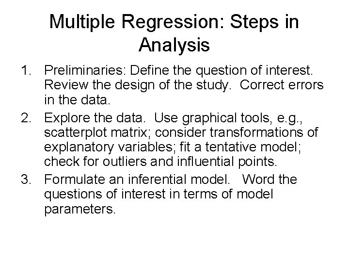
Multiple Regression: Steps in Analysis 1. Preliminaries: Define the question of interest. Review the design of the study. Correct errors in the data. 2. Explore the data. Use graphical tools, e. g. , scatterplot matrix; consider transformations of explanatory variables; fit a tentative model; check for outliers and influential points. 3. Formulate an inferential model. Word the questions of interest in terms of model parameters.

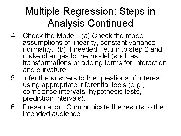
Multiple Regression: Steps in Analysis Continued 4. Check the Model. (a) Check the model assumptions of linearity, constant variance, normality. (b) If needed, return to step 2 and make changes to the model (such as transformations or adding terms for interaction and curvature 5. Infer the answers to the questions of interest using appropriate inferential tools (e. g. , confidence intervals, hypothesis tests, prediction intervals). 6. Presentation: Communicate the results to the intended audience.

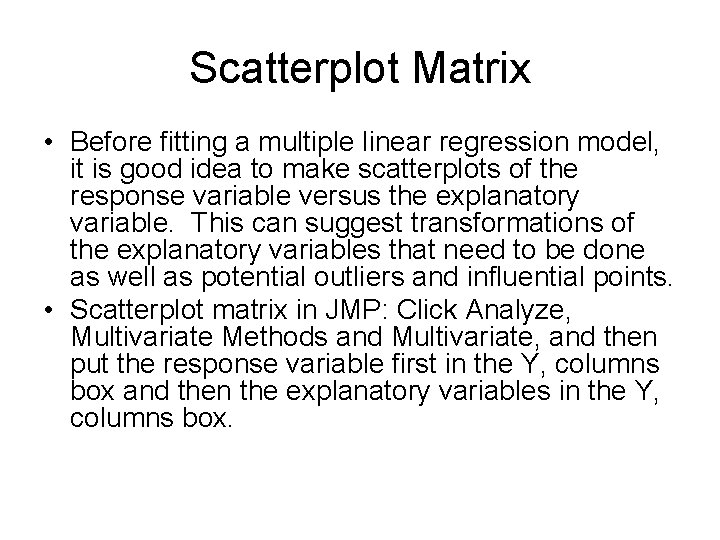
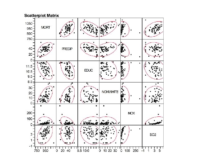
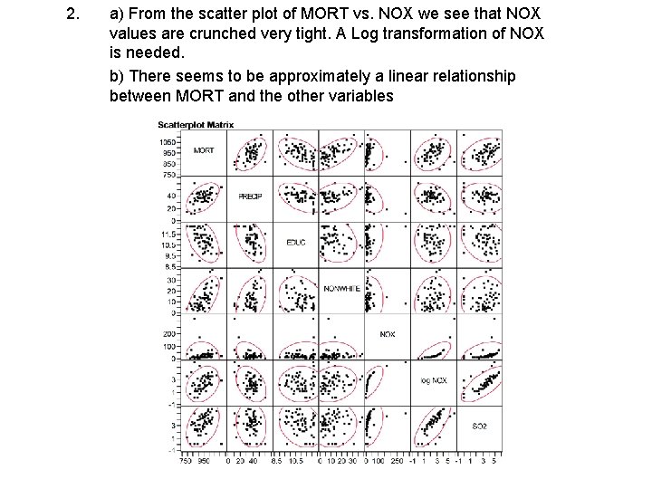
Scatterplot Matrix • Before fitting a multiple linear regression model, it is good idea to make scatterplots of the response variable versus the explanatory variable. This can suggest transformations of the explanatory variables that need to be done as well as potential outliers and influential points. • Scatterplot matrix in JMP: Click Analyze, Multivariate Methods and Multivariate, and then put the response variable first in the Y, columns box and then the explanatory variables in the Y, columns box.

Crunched Variables • When an X variable is “crunched – meaning that most of its values are crunched together and a few are far apart – there will be influential points. To reduce the effects of crunching, it is a good idea to transform the variable to log of the variable.

2. a) From the scatter plot of MORT vs. NOX we see that NOX values are crunched very tight. A Log transformation of NOX is needed. b) There seems to be approximately a linear relationship between MORT and the other variables

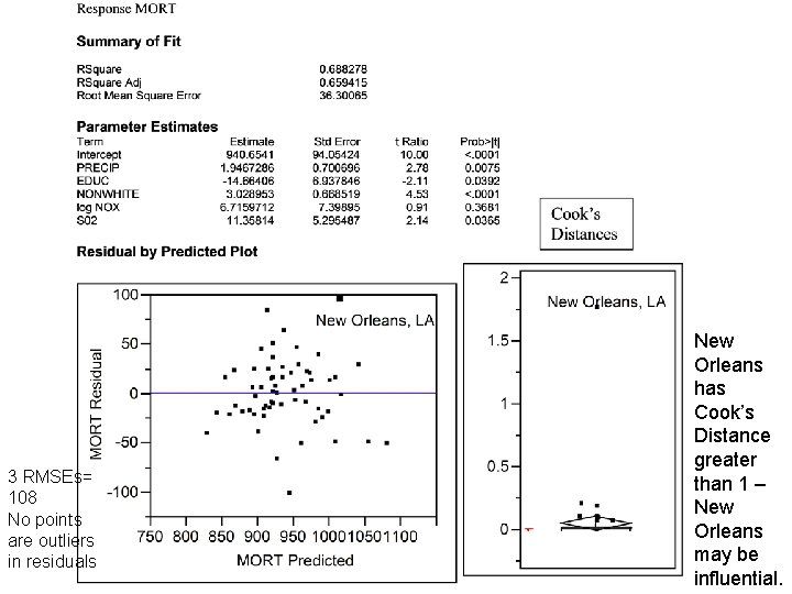
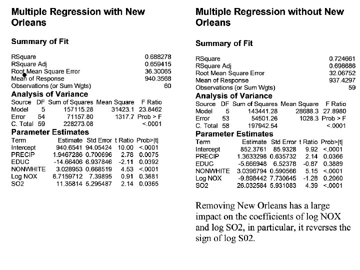
3 RMSEs= 108 No points are outliers in residuals New Orleans has Cook’s Distance greater than 1 – New Orleans may be influential.

Labeling Observations • To have points identified by a certain column, go the column, click Columns and click Label (click Unlabel to Unlabel). • To label a row, go to the row, click rows and click label.

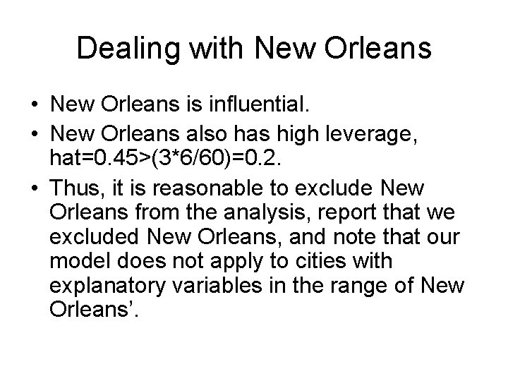
Dealing with New Orleans • New Orleans is influential. • New Orleans also has high leverage, hat=0. 45>(3*6/60)=0. 2. • Thus, it is reasonable to exclude New Orleans from the analysis, report that we excluded New Orleans, and note that our model does not apply to cities with explanatory variables in the range of New Orleans’.