Descriptive Statistics The goal of descriptive statistics is

Descriptive Statistics The goal of descriptive statistics is to summarize a collection of data in a clear and understandable way.

Summary Measures Central Tendency Mean Median Mode Quartile Range Variance Geometric Mean Variation Coefficient of Variation Standard Deviation

INVESTIGATION Data Colllection Data Presentation Tabulation Diagrams Graphs Descriptive Statistics Measures of Location Measures of Dispersion Measures of Skewness & Kurtosis Inferential Statistiscs Estimation Hypothesis Testing Ponit estimate Inteval estimate Univariate analysis Multivariate analysis

Measures of Central Tendency or Measures of Location or Measures of Averages

Central Tendency �Measures of Central Tendency: �Mean � The sum of all scores divided by the number of scores. �Median � The value that divides the distribution in half when observations are ordered. �Mode � The most frequent score.

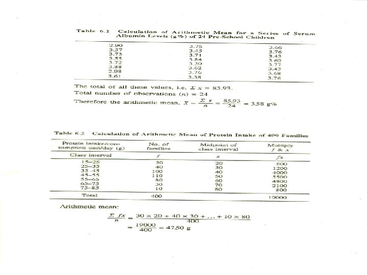
Measure of central tendency Arithmetic Mean (Mean) Definition: Sum of all the observation s divided by the number of the observations The arithmetic mean is the most common measure of the central location of a sample. Population Sample

“sigma”, the sum of X, add up all scores Mean �Population “mu” �Sample “N”, the total number of scores in a population “sigma”, the sum of X, add up all scores “X bar” “n”, the total number of scores in a sample

Mean: Example Data: {1, 3, 6, 7, 2, 3, 5} • number of observations: 7 • Sum of observations: 27 • Mean: 3. 9

Simple Frequency Distributions raw-score distribution name Student 1 Student 2 Student 3 Student 4 Student 5 Student 6 Student 7 Student 8 X 20 23 15 21 15 20 frequency distribution f 3 2 2 1 Mean X 15 20 21 23 c= Sfc N

Mean �Is the balance point of a distribution.

Pros and Cons of the Mean Pros Cons Mathematical center of a distribution. Good for interval and ratio data. Does not ignore any information. Inferential statistics is based on mathematical properties of the mean. Influenced by extreme scores and skewed distributions. May not exist in the data.

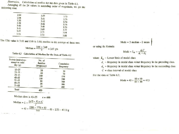
Median Definition: The value that is larger than half the population and smaller than half the population n is odd: the median score 5, 8, 9, 10, 28 median = 9 n is even: the th score 6, 17, 19, 20, 21, 27 median = 19. 5

Pros and Cons of Median Pros Cons Not influenced by extreme scores or skewed distributions. Good with ordinal data. Easier to compute than the mean. May not exist in the data. Doesn’t take actual values into account.

Mode Most frequently occurring value Data • Mode : 3 {1, 3, 7, 3, 2, 3, 6, 7} Data • Mode : 1, 3 {1, 3, 7, 3, 2, 3, 6, 7, 1, 1} Data {1, 3, 7, 0, 2, -3, 6, 5, -1} • Mode : none

Central Tendency Example: Mode � 52, 76, 100, 136, 186, 196, 205, 150, 257, 264, 280, 282, 283, 303, 317, 325, 373, 384, 400, 402, 417, 422, 472, 480, 643, 693, 732, 749, 750, 791, 891 �Mode: most frequent observation �Mode(s) for hotel rates: � 264, 317, 384

Pros and Cons of the Mode Pros Cons Good for nominal & ordinal data. Easiest to compute and understand. The score comes from the data set. Ignores most of the information in a distribution. Small samples may not have a mode.

Example: Central Location Suppose the age in years of the first 10 subjects enrolled in your study are: 34, 24, 56, 52, 21, 44, 64, 34, 42, 46 Then the mean age of this group is 41. 7 years To find the median, first order the data: 21, 24, 34, 42, 44, 46, 52, 56, 64 The median is 42 +44 = 43 years 2 The mode is 34 years.

Comparison of Mean and Median • Mean is sensitive to a few very large (or small) values “outliers” so sometime mean does not reflect the quantity desired. • Median is “resistant” to outliers • Mean is attractive mathematically

Suppose the next patient enrolls and their age is 97 years. How does the mean and median change? To get the median, order the data: 21, 24, 34, 42, 44, 46, 52, 56, 64, 97 If the age were recorded incorrectly as 977 instead of 97, what would the new median be? What would the new mean be?

Calculating the Mean from a Frequency Distribution

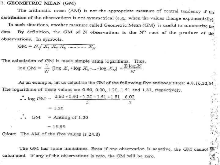
MEASURES OF Central Tendency Geometric Mean & Harmonic Mean

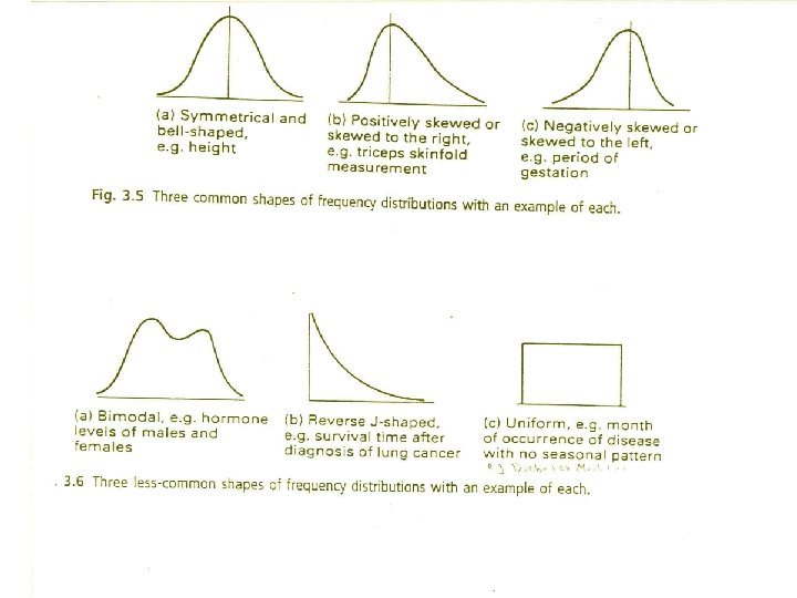
The Shape of Distributions �Distributions can be either symmetrical or skewed, depending on whethere are more frequencies at one end of the distribution than the other.

Symmetrical Distributions �A distribution is symmetrical if the frequencies at the right and left tails of the distribution are identical, so that if it is divided into two halves, each will be the mirror image of the other. � In a symmetrical distribution the mean, median, and mode are identical.

Almost Symmetrical distribution Mean= 13. 4 Mode= 13. 0

Skewed Distribution Few extreme values on one side of the distribution or on the other. �Positively skewed distributions: distributions which have few extremely high values (Mean>Median) �Negatively skewed distributions: distributions which have few extremely low values(Mean<Median)

Positively Skewed Distribution Mean=1. 13 Median=1. 0

Negatively Skewed distribution Mean=3. 3 Median=4. 0

Mean, Median and Mode

Distributions Bell-Shaped (also known as symmetric” or “normal”) Skewed: positively (skewed to the right) – it tails off toward larger values negatively (skewed to the left) – it tails off toward smaller values

Choosing a Measure of Central Tendency �IF variable is Nominal. . �Mode �IF variable is Ordinal. . . �Mode or Median(or both) �IF variable is Interval-Ratio and distribution is Symmetrical… �Mode, Median or Mean �IF variable is Interval-Ratio and distribution is Skewed… �Mode or Median

EXAMPLE: (1) 7, 8, 9, 10, 11 n=5, x=45, =45/5=9 (2) 3, 4, 9, 12, 15 n=5, x=45, =45/5=9 (3) 1, 5, 9, 13, 17 n=5, x=45, =45/5=9 S. D. : (1) 1. 58 (2) 4. 74 (3) 6. 32