Measurement Math De Shon 2006 Univariate Descriptives n

Measurement Math De. Shon - 2006

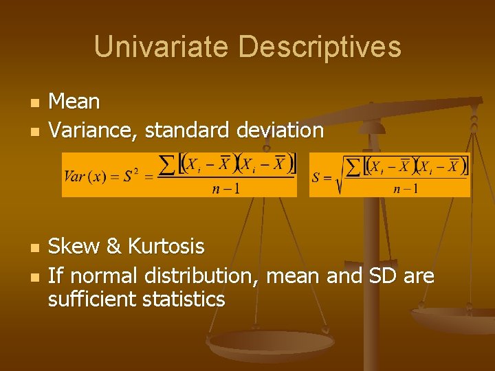
Univariate Descriptives n n Mean Variance, standard deviation Skew & Kurtosis If normal distribution, mean and SD are sufficient statistics

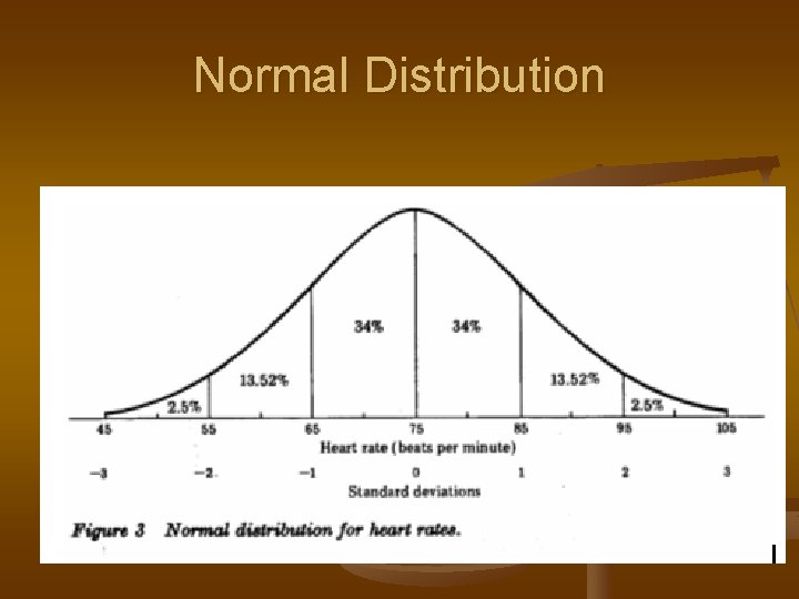
Normal Distribution

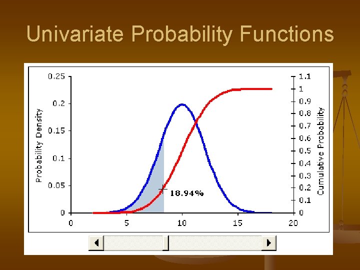
Univariate Probability Functions

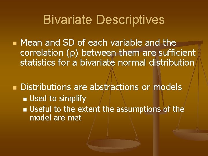
Bivariate Descriptives n n Mean and SD of each variable and the correlation (ρ) between them are sufficient statistics for a bivariate normal distribution Distributions are abstractions or models Used to simplify n Useful to the extent the assumptions of the model are met n

2 D – Ellipse or Scatterplot Galton’s Original Graph

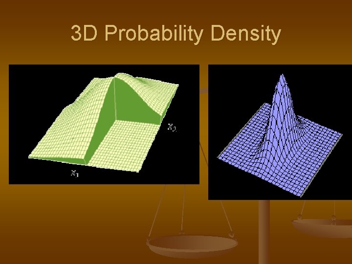
3 D Probability Density

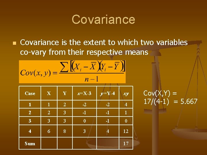
Covariance n Covariance is the extent to which two variables co-vary from their respective means Case X Y x=X-3 y =Y-4 xy 1 1 2 -2 -2 4 2 2 3 -1 -1 1 3 3 3 0 -1 0 4 6 8 3 4 12 Sum 17 Cov(X, Y) = 17/(4 -1) = 5. 667

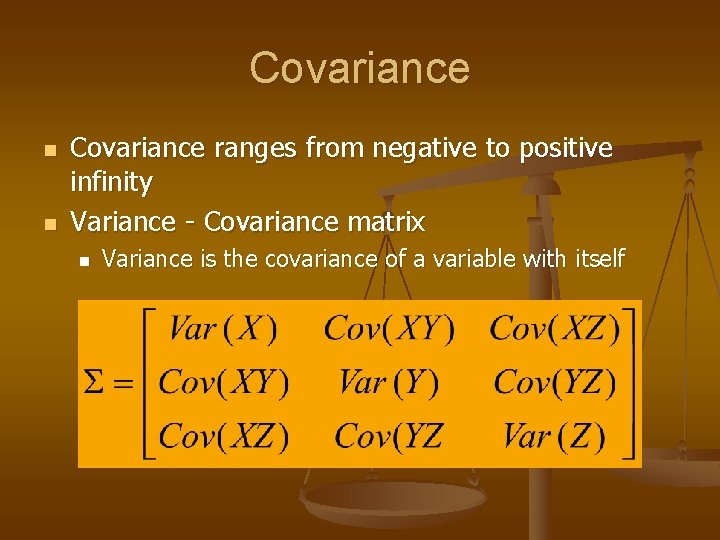
Covariance n n Covariance ranges from negative to positive infinity Variance - Covariance matrix n Variance is the covariance of a variable with itself

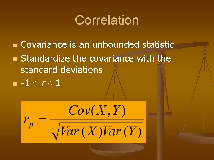
Correlation n Covariance is an unbounded statistic Standardize the covariance with the standard deviations -1 ≤ r ≤ 1

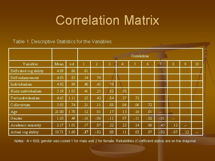
Correlation Matrix Table 1. Descriptive Statistics for the Variables Correlations Variables Mean s. d 1 2 3 4 5 6 7 8 Self-rated cog ability 4. 89 . 86 . 81 Self-enhancement 4. 03 . 85 . 34 . 79 Individualism 4. 92 . 89 . 40 . 41 . 78 Horiz individualism 5. 19 1. 05 . 41 . 25 . 82 . 80 Vert individualism 4. 65 1. 11 . 25 . 42 . 84 . 37 . 72 Collectivism 5. 05 . 74 . 21 . 11 . 08 . 06 . 72 21. 00 1. 70 . 12 . 01 . 17 . 13 . 16 . 01 -- Gender 1. 63 . 49 -. 16 -. 06 -. 11 . 07 -. 11 -. 02 -. 01 Academic seniority 2. 17 1. 01 . 17 . 07 . 22 . 23 . 14 . 06 . 45 . 12 10. 71 1. 60 . 17 -. 02 . 08 . 11 . 03 . 07 -. 02 -. 07 Age Actual cog ability 9 10 --. 12 -- Notes: N = 608; gender was coded 1 for male and 2 for female. Reliabilities (Coefficient alpha) are on the diagonal.

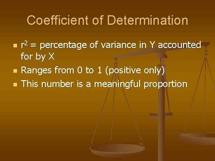
Coefficient of Determination n r 2 = percentage of variance in Y accounted for by X Ranges from 0 to 1 (positive only) This number is a meaningful proportion

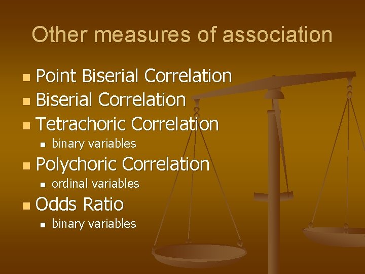
Other measures of association Point Biserial Correlation n Tetrachoric Correlation n Polychoric Correlation n n binary variables ordinal variables Odds Ratio n binary variables

Point Biserial Correlation n n Used when one variable is a natural (real) dichotomy (two categories) and the other variable is interval or continuous Just a normal correlation between a continuous and a dichotomous variable

Biserial Correlation n When one variable is an artificial dichotomy (two categories) and the criterion variable is interval or continuous

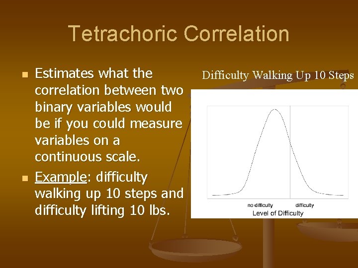
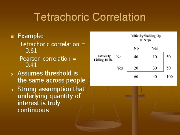
Tetrachoric Correlation n n Estimates what the correlation between two binary variables would be if you could measure variables on a continuous scale. Example: difficulty walking up 10 steps and difficulty lifting 10 lbs. Difficulty Walking Up 10 Steps

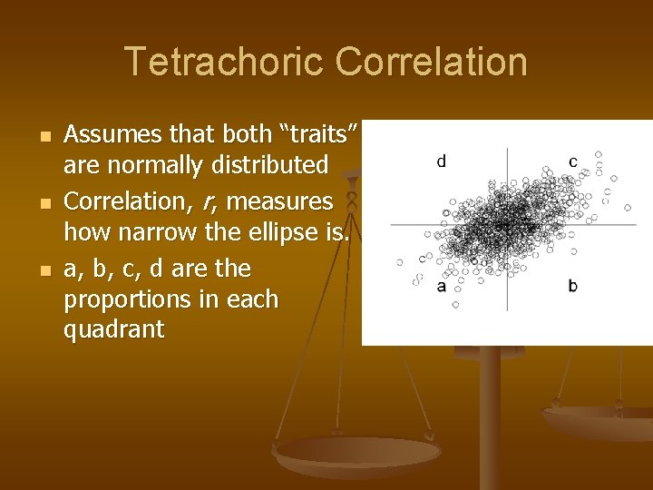
Tetrachoric Correlation n Assumes that both “traits” are normally distributed Correlation, r, measures how narrow the ellipse is. a, b, c, d are the proportions in each quadrant

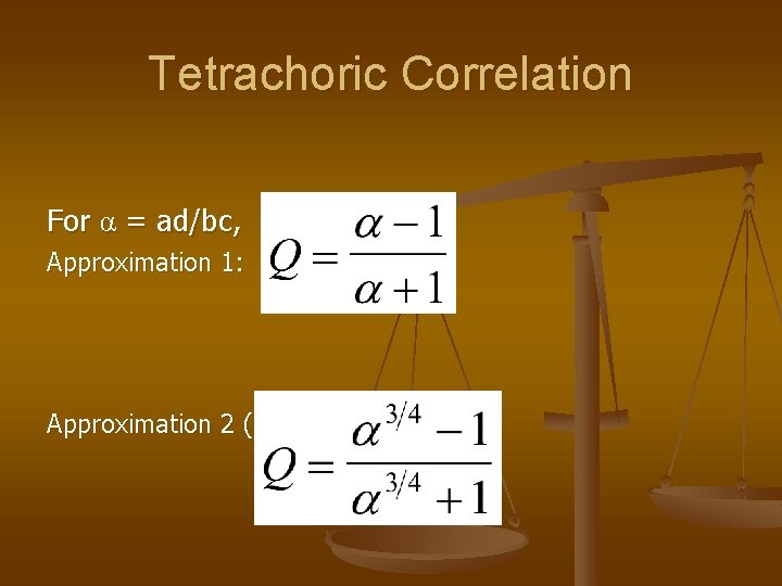
Tetrachoric Correlation For α = ad/bc, Approximation 1: Approximation 2 (Digby):

Tetrachoric Correlation n Example: Tetrachoric correlation = 0. 61 Pearson correlation = 0. 41 o o Assumes threshold is the same across people Strong assumption that underlying quantity of interest is truly continuous

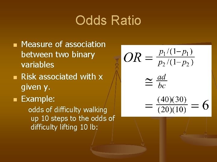
Odds Ratio n n n Measure of association between two binary variables Risk associated with x given y. Example: odds of difficulty walking up 10 steps to the odds of difficulty lifting 10 lb:

Pros and Cons n Tetrachoric correlation n n Odds Ratio n n same interpretation as Spearman and Pearson correlations “difficult” to calculate exactly Makes assumptions easy to understand, but no “perfect” association that is manageable (i. e. {∞, -∞}) easy to calculate not comparable to correlations May give you different results/inference!

Dichotomized Data: A Bad Habit of Psychologists n Sometimes perfectly good quantitative data is made binary because it seems easier to talk about "High" vs. "Low" n The worst habit is median split n n n Usually the High and Low groups are mixtures of the continua Rarely is the median interpreted rationally See references n n Cohen, J. (1983) The cost of dichotomization. Applied Psychological Measurement, 7, 249 -253. Mc. Callum, R. C. , Zhang, S. , Preacher, K. J. , Rucker, D. D. (2002) On the practice of dichotomization of quantitative variables. Psychological Methods, 7, 19 -40.

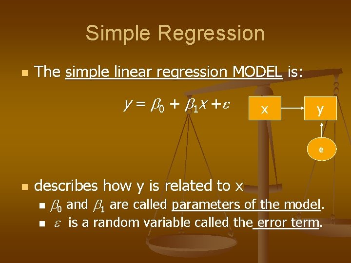
Simple Regression n The simple linear regression MODEL is: y = b 0 + b 1 x + x y e n describes how y is related to x b 0 and b 1 are called parameters of the model. n is a random variable called the error term. n

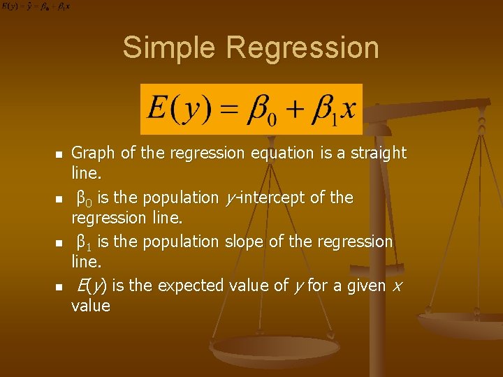
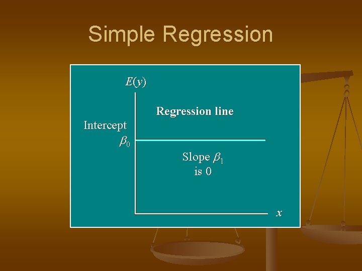
Simple Regression n n Graph of the regression equation is a straight line. β 0 is the population y-intercept of the regression line. β 1 is the population slope of the regression line. E(y) is the expected value of y for a given x value

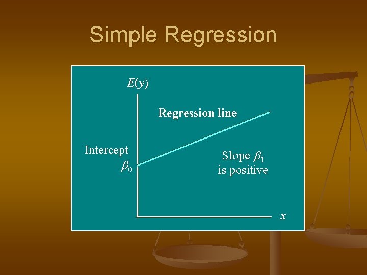
Simple Regression E (y ) Regression line Intercept b 0 Slope b 1 is positive x

Simple Regression E (y ) Regression line Intercept b 0 Slope b 1 is 0 x

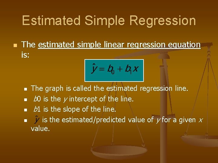
Estimated Simple Regression n The estimated simple linear regression equation is: n n The graph is called the estimated regression line. b 0 is the y intercept of the line. b 1 is the slope of the line. is the estimated/predicted value of y for a given x value.

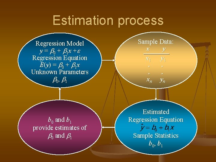
Estimation process Regression Model y = b 0 + b 1 x + Regression Equation E(y) = b 0 + b 1 x Unknown Parameters b 0, b 1 b 0 and b 1 provide estimates of b 0 and b 1 Sample Data: x y x 1 y 1. . xn yn Estimated Regression Equation Sample Statistics b 0, b 1

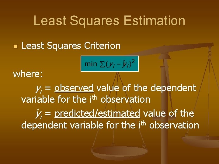
Least Squares Estimation n Least Squares Criterion where: yi = observed value of the dependent variable for the ith observation ^ yi = predicted/estimated value of the dependent variable for the ith observation

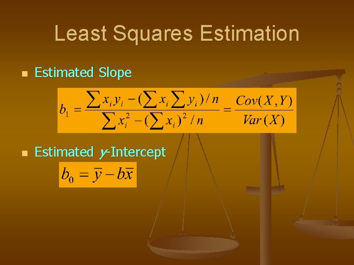
Least Squares Estimation n Estimated Slope n Estimated y-Intercept

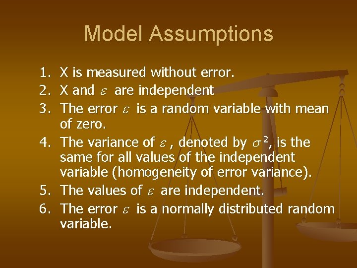
Model Assumptions 1. 2. 3. 4. 5. 6. X is measured without error. X and are independent The error is a random variable with mean of zero. The variance of , denoted by 2, is the same for all values of the independent variable (homogeneity of error variance). The values of are independent. The error is a normally distributed random variable.

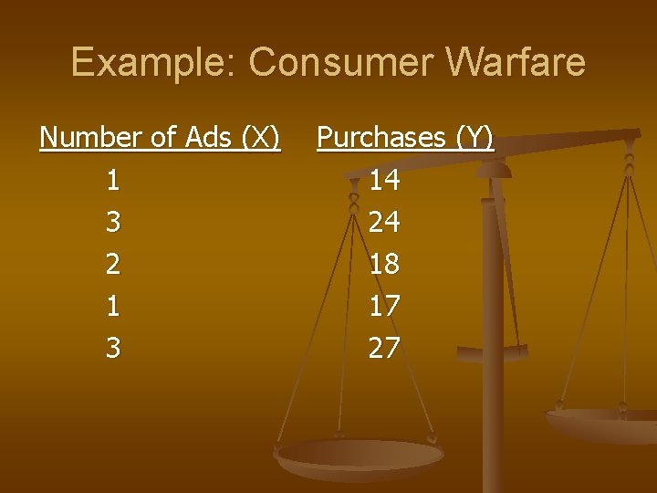
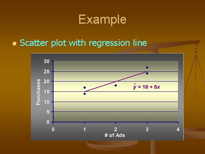
Example: Consumer Warfare Number of Ads (X) 1 3 2 1 3 Purchases (Y) 14 24 18 17 27

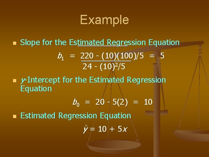
Example n Slope for the Estimated Regression Equation b 1 = 220 - (10)(100)/5 = 5 24 - (10)2/5 n y-Intercept for the Estimated Regression Equation b 0 = 20 - 5(2) = 10 n Estimated Regression Equation y^ = 10 + 5 x

Example n Scatter plot with regression line ^

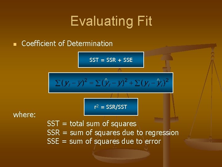
Evaluating Fit n Coefficient of Determination SST = SSR + SSE ^ where: ^ r 2 = SSR/SST = total sum of squares SSR = sum of squares due to regression SSE = sum of squares due to error

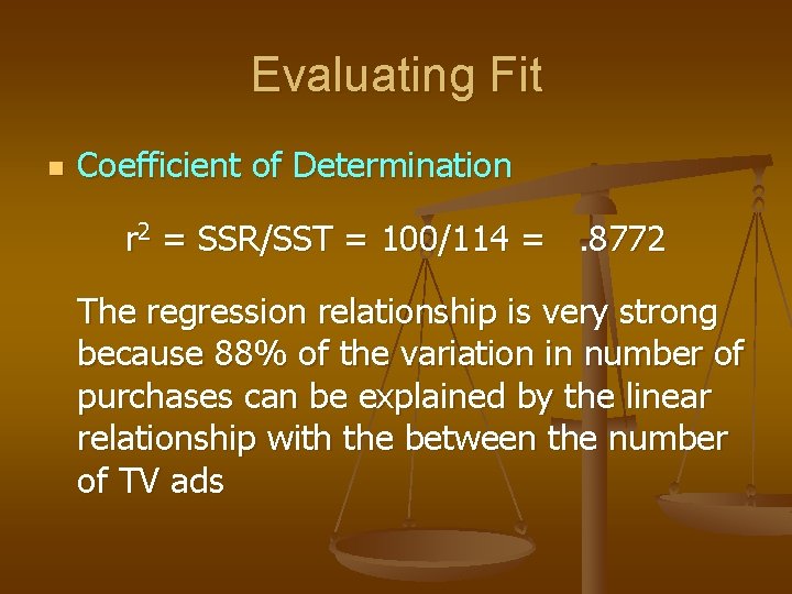
Evaluating Fit n Coefficient of Determination r 2 = SSR/SST = 100/114 =. 8772 The regression relationship is very strong because 88% of the variation in number of purchases can be explained by the linear relationship with the between the number of TV ads

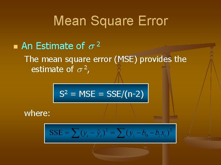
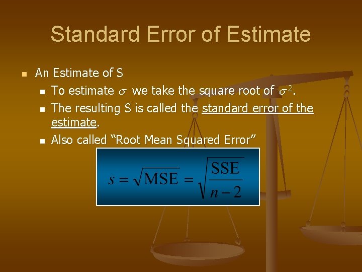
Mean Square Error n An Estimate of 2 The mean square error (MSE) provides the estimate of 2, S 2 = MSE = SSE/(n-2) where:

Standard Error of Estimate n An Estimate of S n To estimate we take the square root of 2. n The resulting S is called the standard error of the estimate. n Also called “Root Mean Squared Error”

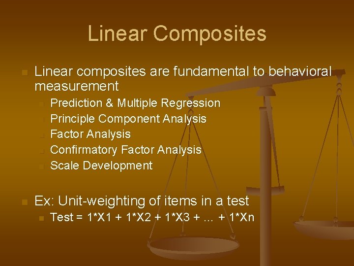
Linear Composites n Linear composites are fundamental to behavioral measurement n n n Prediction & Multiple Regression Principle Component Analysis Factor Analysis Confirmatory Factor Analysis Scale Development Ex: Unit-weighting of items in a test n Test = 1*X 1 + 1*X 2 + 1*X 3 + … + 1*Xn

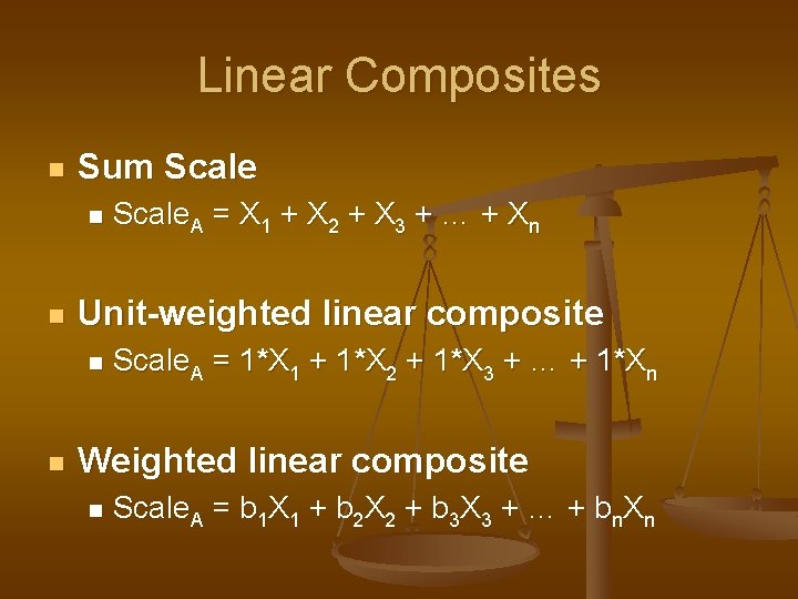
Linear Composites n Sum Scale n n Unit-weighted linear composite n n Scale. A = X 1 + X 2 + X 3 + … + Xn Scale. A = 1*X 1 + 1*X 2 + 1*X 3 + … + 1*Xn Weighted linear composite n Scale. A = b 1 X 1 + b 2 X 2 + b 3 X 3 + … + bn. Xn

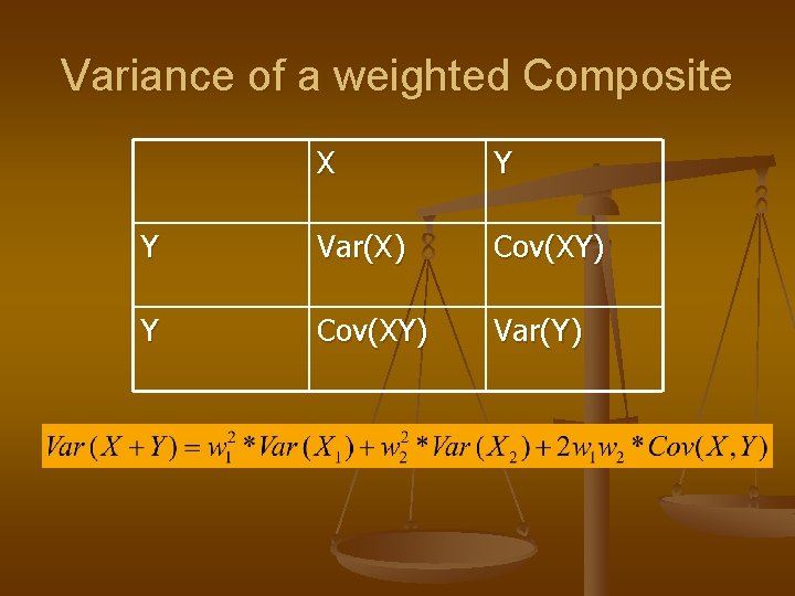
Variance of a weighted Composite X Y Y Var(X) Cov(XY) Y Cov(XY) Var(Y)

Effective vs. Nominal Weights n Nominal weights n n The desired weight assigned to each component Effective weights the actual contribution of each component to the composite n function of the desired weights, standard deviations, and covariances of the components n

Principles of Composite Formation n n Standardize before combining!!!!! Weighting doesn’t matter much when the correlations among the components are moderate to large As the number of components increases, the importance of weighting decreases Differential weights are difficult to replicate/cross-validate

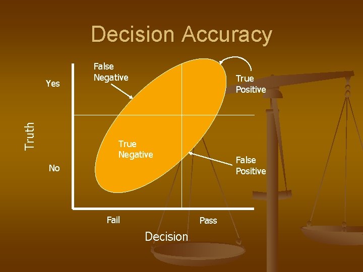
Decision Accuracy Truth Yes False Negative True Positive True Negative False Positive No Fail Pass Decision

Signal Detection Theory

Polygraph Example n Sensitivity, etc…