Item Response Theory Psych 818 De Shon IRT

Item Response Theory Psych 818 De. Shon

IRT ● Typically used for 0, 1 data (yes, no; correct, incorrect) – – – ● Set of probabilistic models that… Describes the relationship between a respondent’s level on a construct (a. k. a. latent trait; e. g. , extraversion, cognitive ability, affective commitment)… To his or her probability of a particular response to an individual item Samejima's Graded Response model – For polytomous data where options are ordered along a continuum (e. g. , Likert scales)

Advantages of IRT? ● Provides more information than classical test theory (CTT) – – ● ● Classical test statistics depend on the set of items and sample examined IRT modelling not dependent on sample examined Can examine item bias/ measurement equivalence SEM’s vary at different levels of the trait (conditional standard errors of measurement) Used to estimate item parameters (e. g. , difficulty and discrimination) and. . . Person true scores on the latent trait

Advantages of IRT? ● Invariance of IRT Parameters – Difficulty and Discrimination parameters for an item are invariant across populations ● Within a linear transformation – That is no matter who you administer the test to, you should get the same item parameters – However, precision of estimates will differ ● If there is little variance on an item in a sample with have unstable parameter estimates

IRT Assumptions ● ● Underlying trait or ability (continuous) Latent trait is normally distributed Items are unidimensional Local Independence – ● if remove common factor the items are uncorrelated Items can be allowed to vary with respect to: – – – Difficulty (one parameter model; Rasch model) Discriminability (two parameter model) Guessing (three parameter model)

Model Setup ● ● Consider a test with p binary (correct/incorrect) responses Each item is assumed to ‘reflect’ one underlying (latent) dimensions of ‘achievement’ or ‘ability’ Start with an assumed 1 -dimensional test, say of sexual attitude mathematics with 10 items. How do we get a value (score) on the mathematics scale from a set of 40 (1/0) responses from each individual? Set up a Model. .

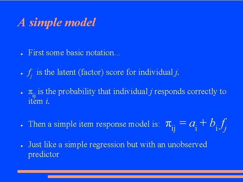
A simple model ● First some basic notation. . . ● fj is the latent (factor) score for individual j. ● ● ● πij is the probability that individual j responds correctly to item i. Then a simple item response model is: πij = ai + bi fj Just like a simple regression but with an unobserved predictor

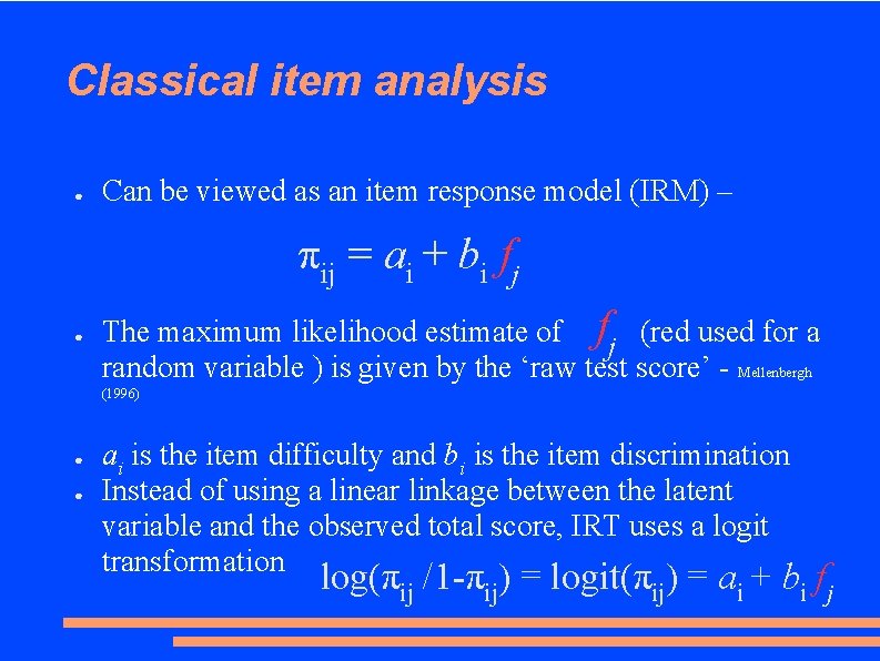
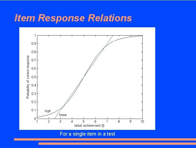
Classical item analysis ● Can be viewed as an item response model (IRM) – πij = ai + bi fj ● The maximum likelihood estimate of fj (red used for a random variable ) is given by the ‘raw test score’ - Mellenbergh (1996) ● ● ai is the item difficulty and bi is the item discrimination Instead of using a linear linkage between the latent variable and the observed total score, IRT uses a logit transformation log(πij /1 -πij) = logit(πij) = ai + bi fj

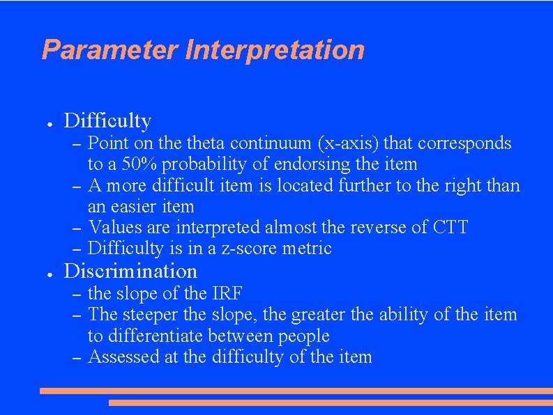
Parameter Interpretation ● Difficulty – – ● Point on theta continuum (x-axis) that corresponds to a 50% probability of endorsing the item A more difficult item is located further to the right than an easier item Values are interpreted almost the reverse of CTT Difficulty is in a z-score metric Discrimination – – – the slope of the IRF The steeper the slope, the greater the ability of the item to differentiate between people Assessed at the difficulty of the item

Item Response Relations For a single item in a test

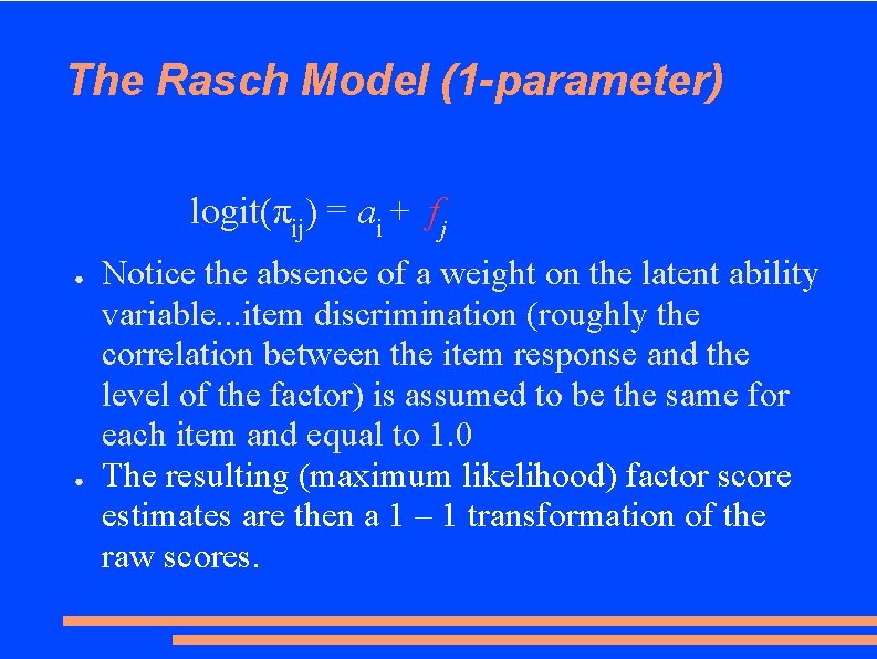
The Rasch Model (1 -parameter) logit(πij) = ai + fj ● ● Notice the absence of a weight on the latent ability variable. . . item discrimination (roughly the correlation between the item response and the level of the factor) is assumed to be the same for each item and equal to 1. 0 The resulting (maximum likelihood) factor score estimates are then a 1 – 1 transformation of the raw scores.

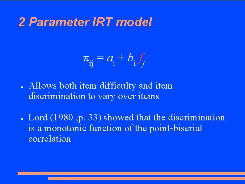
2 Parameter IRT model πij = ai + bi fj ● ● Allows both item difficulty and item discrimination to vary over items Lord (1980 , p. 33) showed that the discrimination is a monotonic function of the point-biserial correlation

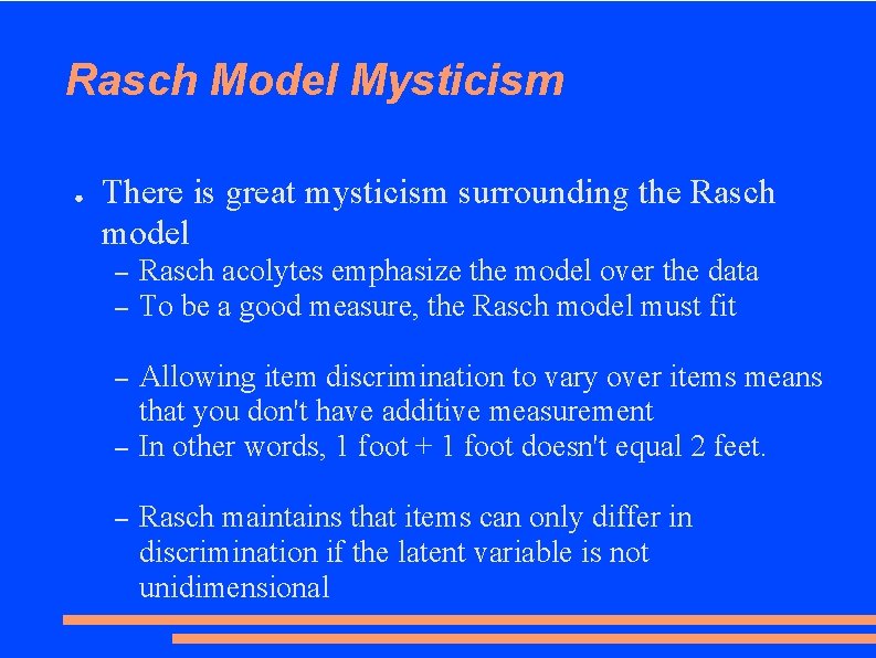
Rasch Model Mysticism ● There is great mysticism surrounding the Rasch model – – Rasch acolytes emphasize the model over the data To be a good measure, the Rasch model must fit – Allowing item discrimination to vary over items means that you don't have additive measurement In other words, 1 foot + 1 foot doesn't equal 2 feet. – – Rasch maintains that items can only differ in discrimination if the latent variable is not unidimensional

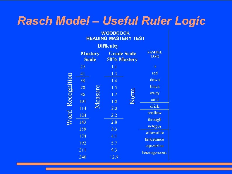
Rasch Model – Useful Ruler Logic

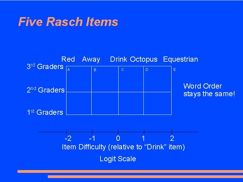
Five Rasch Items Red Away 3 rd Graders A B Drink Octopus Equestrian C D E Word Order stays the same! 2 nd Graders 1 st Graders -2 -1 0 1 2 Item Difficulty (relative to “Drink” item) Logit Scale

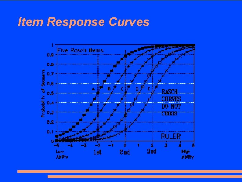
Item Response Curves

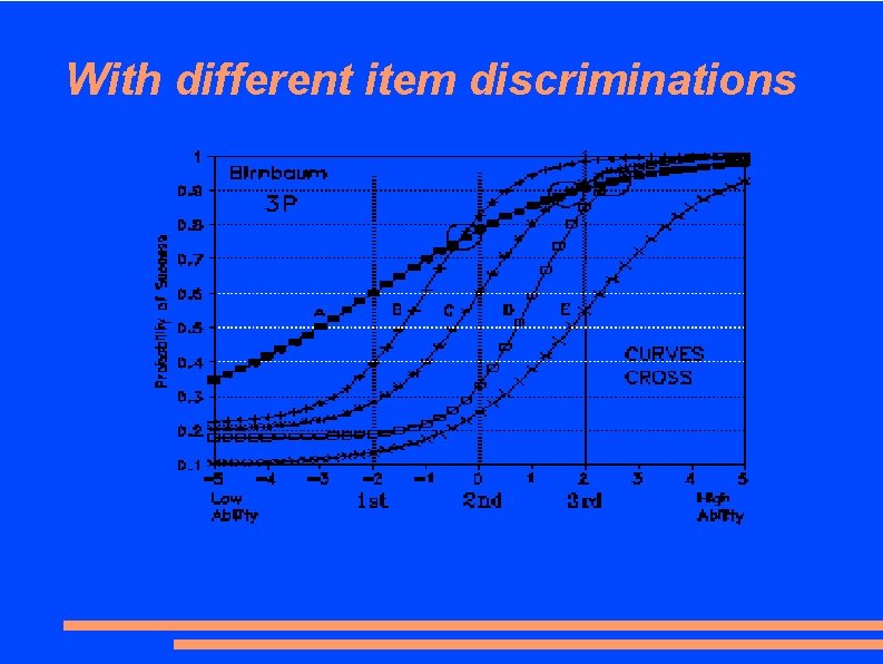
With different item discriminations

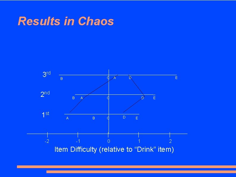
Results in Chaos 3 rd C B 2 nd 1 st -2 A B A D E D C B -1 A C 0 D E E 1 2 Item Difficulty (relative to “Drink” item)

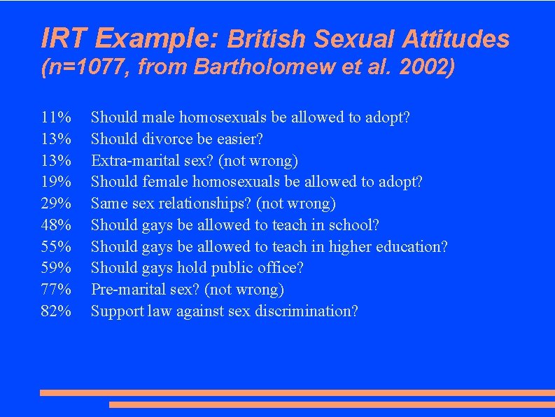
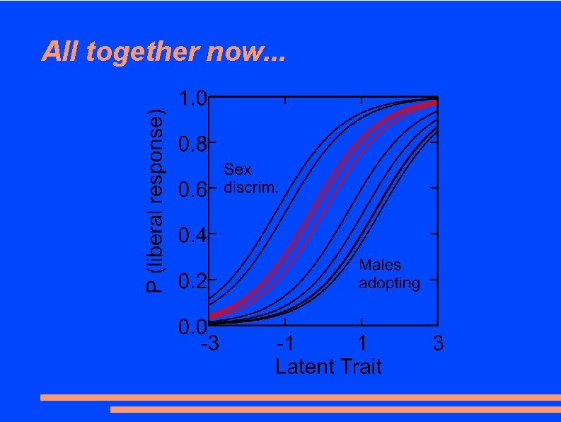
IRT Example: British Sexual Attitudes (n=1077, from Bartholomew et al. 2002) 11% 13% 19% 29% 48% 55% 59% 77% 82% Should male homosexuals be allowed to adopt? Should divorce be easier? Extra-marital sex? (not wrong) Should female homosexuals be allowed to adopt? Same sex relationships? (not wrong) Should gays be allowed to teach in school? Should gays be allowed to teach in higher education? Should gays hold public office? Pre-marital sex? (not wrong) Support law against sex discrimination?

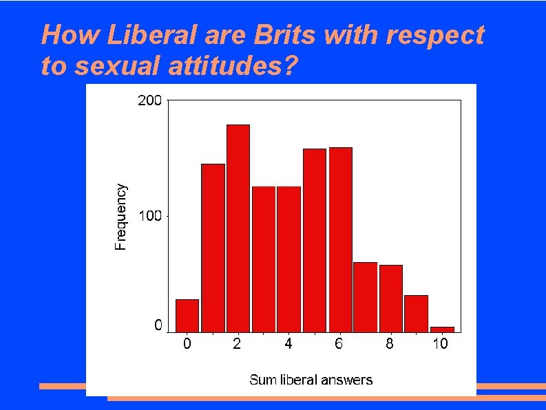
How Liberal are Brits with respect to sexual attitudes?

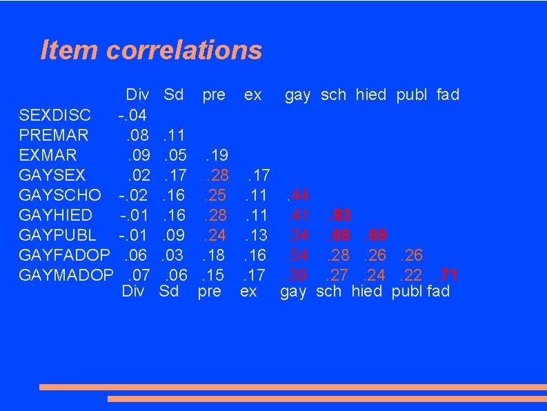
Item correlations Div SEXDISC -. 04 PREMAR. 08 EXMAR. 09 GAYSEX. 02 GAYSCHO -. 02 GAYHIED -. 01 GAYPUBL -. 01 GAYFADOP. 06 GAYMADOP. 07 Div Sd pre ex gay sch hied publ fad . 11. 05. 17. 16. 09. 03. 06 Sd . 19. 28. 25. 28. 24. 18. 15 pre . 17. 11. 13. 16. 17 ex . 44. 41. 83. 34. 66. 69. 34. 28. 26. 39. 27. 24. 22. 71 gay sch hied publ fad

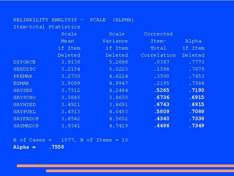
RELIABILITY ANALYSIS Item-total Statistics Scale Mean if Item Deleted DIVORCE 3. 9136 SEXDISC 3. 2154 PREMAR 3. 2730 EXMAR 3. 9099 GAYSEX 3. 7512 GAYSCHO 3. 5645 GAYHIED 3. 4921 GAYPUBL 3. 4513 GAYFADOP 3. 8542 GAYMADOP 3. 9341 SCALE (ALPHA) Scale Variance if Item Deleted 5. 2686 5. 0223 4. 6224 4. 9947 4. 2484 3. 8650 3. 8691 4. 0453 4. 5652 4. 7419 N of Cases = 1077, N of Items = 10 Alpha =. 7558 Corrected Item. Total Correlation. 0387. 1588. 3500. 2195. 5265. 6736. 6743. 5809. 4340. 4486 Alpha if Item Deleted. 7773. 7679. 7453. 7588. 7190. 6915. 7088. 7338. 7349

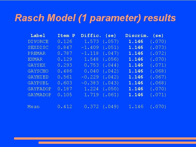
Rasch Model (1 parameter) results Label DIVORCE SEXDISC PREMAR EXMAR GAYSEX GAYSCHO GAYHIED GAYPUBL GAYFADOP GAYMADOP Item P 0. 126 0. 847 0. 787 0. 129 0. 293 0. 486 0. 561 0. 603 0. 187 0. 105 Mean 0. 412 Diffic. (se) 1. 573 (. 057) -1. 409 (. 051) -1. 118 (. 047) 1. 548 (. 056) 0. 753 (. 044) 0. 040 (. 042) -0. 229 (. 042) -0. 383 (. 043) 1. 224 (. 050) 1. 719 (. 061) 0. 372 (. 049) Discrim. (se) 1. 146 (. 070) 1. 146 (. 073) 1. 146 (. 072) 1. 146 (. 070) 1. 146 (. 071) 1. 146 (. 068) 1. 146 (. 067) 1. 146 (. 068) 1. 146 (. 070) 1. 146 (. 071) 1. 146 (. 070)

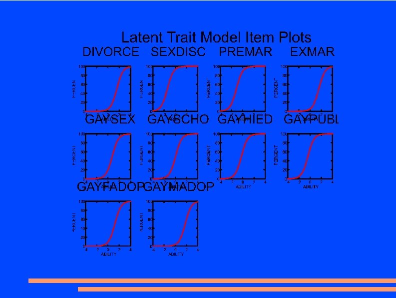
All together now. . .

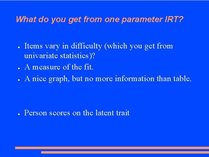
What do you get from one parameter IRT? ● Items vary in difficulty (which you get from univariate statistics)? A measure of the fit. A nice graph, but no more information than table. ● Person scores on the latent trait ● ●

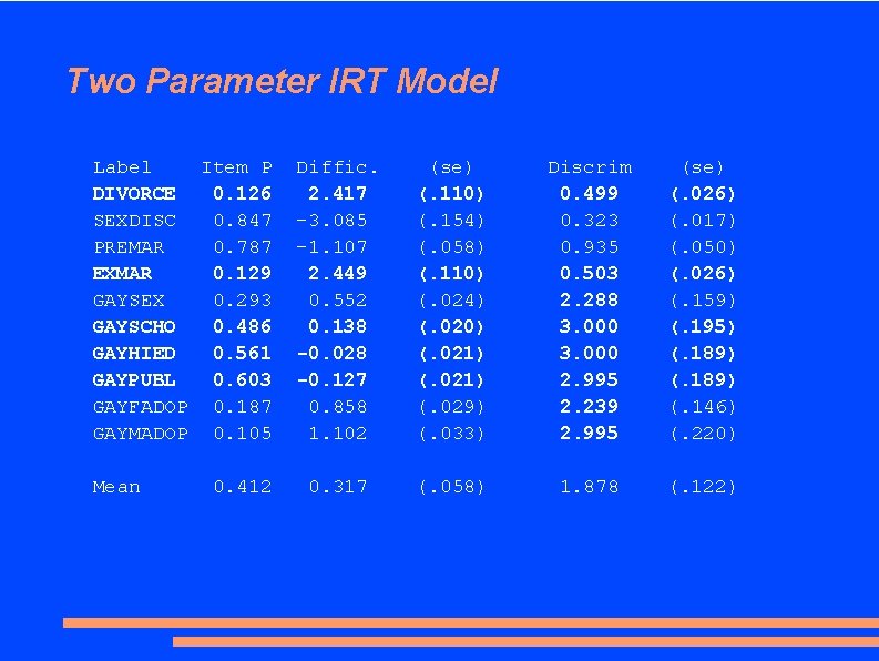
Two Parameter IRT Model Label Item P DIVORCE 0. 126 SEXDISC 0. 847 PREMAR 0. 787 EXMAR 0. 129 GAYSEX 0. 293 GAYSCHO 0. 486 GAYHIED 0. 561 GAYPUBL 0. 603 GAYFADOP 0. 187 GAYMADOP 0. 105 Mean 0. 412 Diffic. 2. 417 -3. 085 -1. 107 2. 449 0. 552 0. 138 -0. 028 -0. 127 0. 858 1. 102 (se) (. 110) (. 154) (. 058) (. 110) (. 024) (. 020) (. 021) (. 029) (. 033) Discrim 0. 499 0. 323 0. 935 0. 503 2. 288 3. 000 2. 995 2. 239 2. 995 (se) (. 026) (. 017) (. 050) (. 026) (. 159) (. 195) (. 189) (. 146) (. 220) 0. 317 (. 058) 1. 878 (. 122)

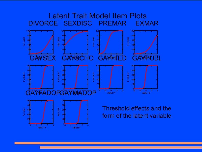
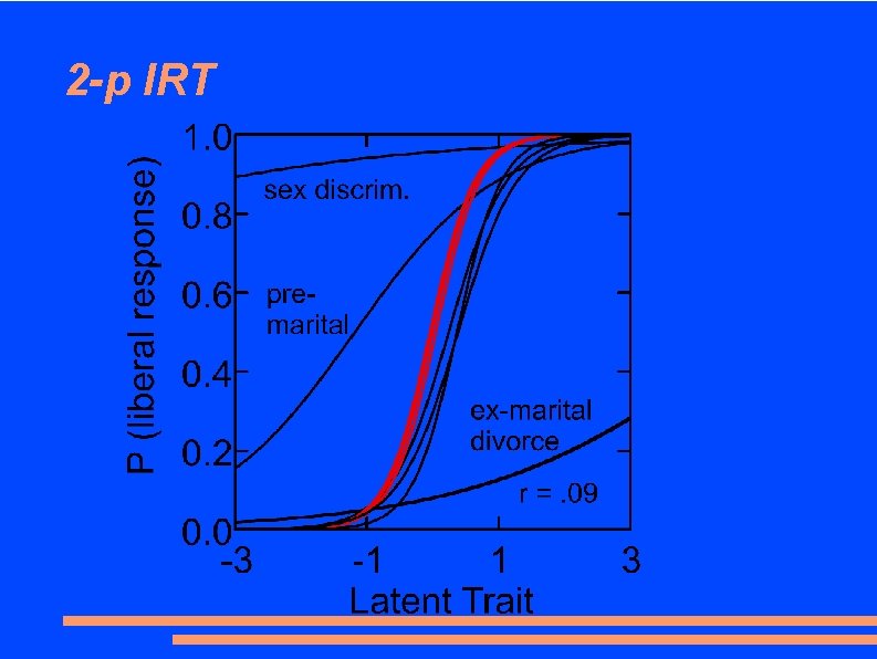
Threshold effects and the form of the latent variable.

2 -p IRT

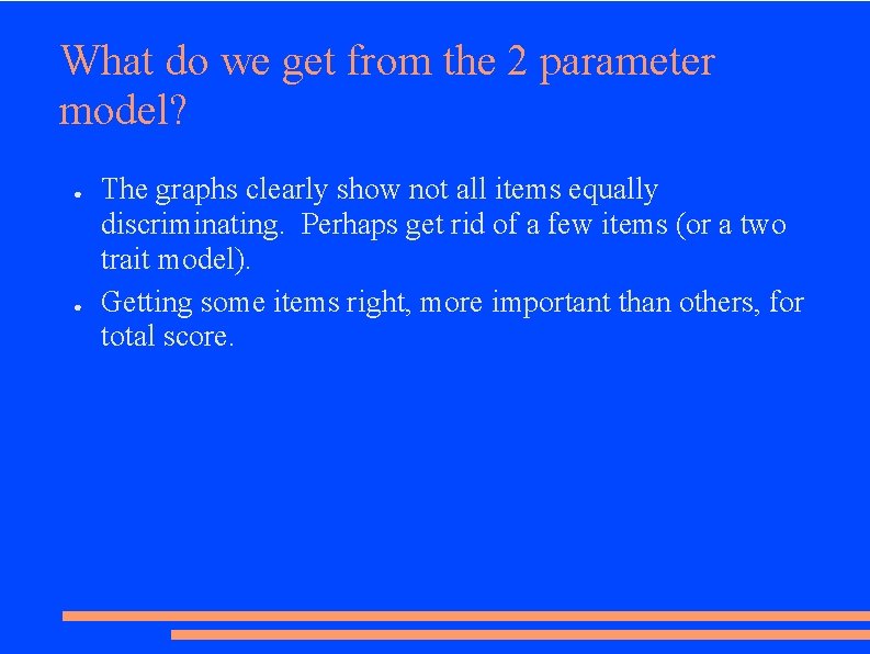
What do we get from the 2 parameter model? ● ● The graphs clearly show not all items equally discriminating. Perhaps get rid of a few items (or a two trait model). Getting some items right, more important than others, for total score.

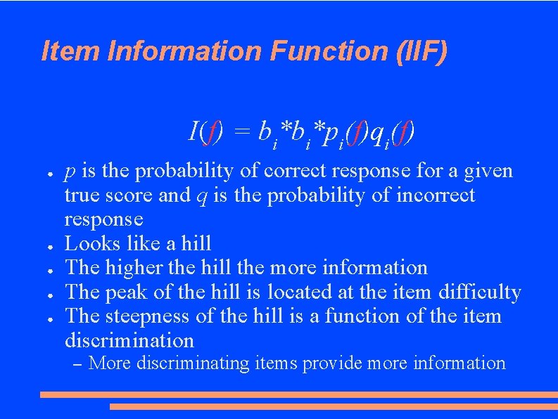
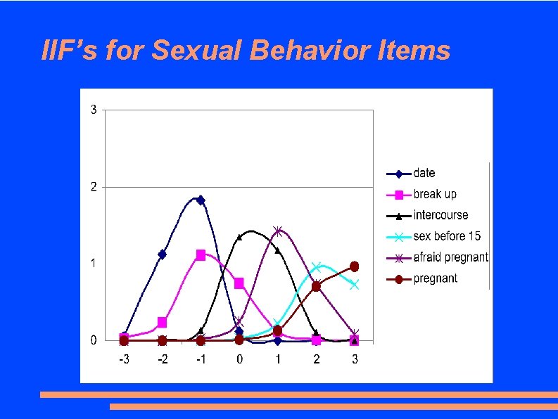
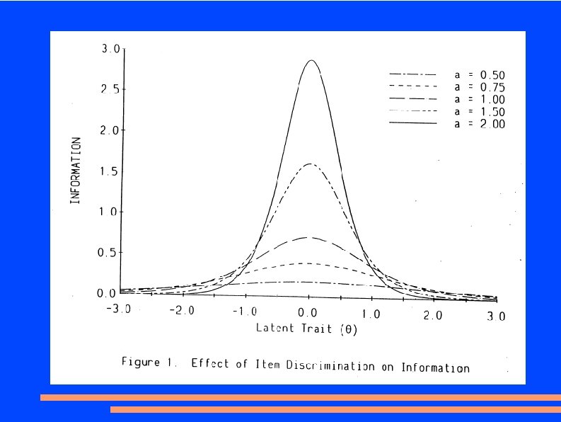
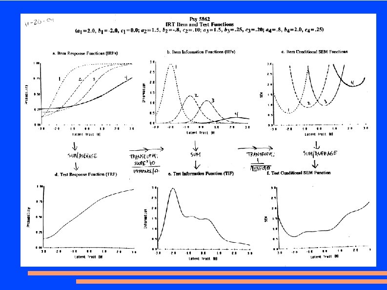
Item Information Function (IIF) I(f) = bi*bi*pi(f)qi(f) ● ● ● p is the probability of correct response for a given true score and q is the probability of incorrect response Looks like a hill The higher the hill the more information The peak of the hill is located at the item difficulty The steepness of the hill is a function of the item discrimination – More discriminating items provide more information

IIF’s for Sexual Behavior Items

Item Standard Error of Measurement (SEM) Function ● ● Estimate of measurement precision at a given theta value SEM = inverse of the square root of the item information SEM is smallest at the item difficulty Items with greater discrimination have smaller SEM, greater measurement precision

Test Information Function (TIF) ● ● ● Sum of all the item information functions Index of how much information a test is providing a given trait level The more items at a given trait level the more information

Test Standard Error of Measurement (SEM) function ● ● Inverse of the square root of the test information function Index of how well, i. e. , precise a test measure’s the trait at a given difficulty level

Check out this for more info ● www 2. uni-jena. de/svw/metheval/irt/Visual. IRT. pdf – Great site with graphical methods for demonstrating the concepts

Testing Model Assumptions ● Unidimensionality ● Model fit – More on this later when we get to CFA

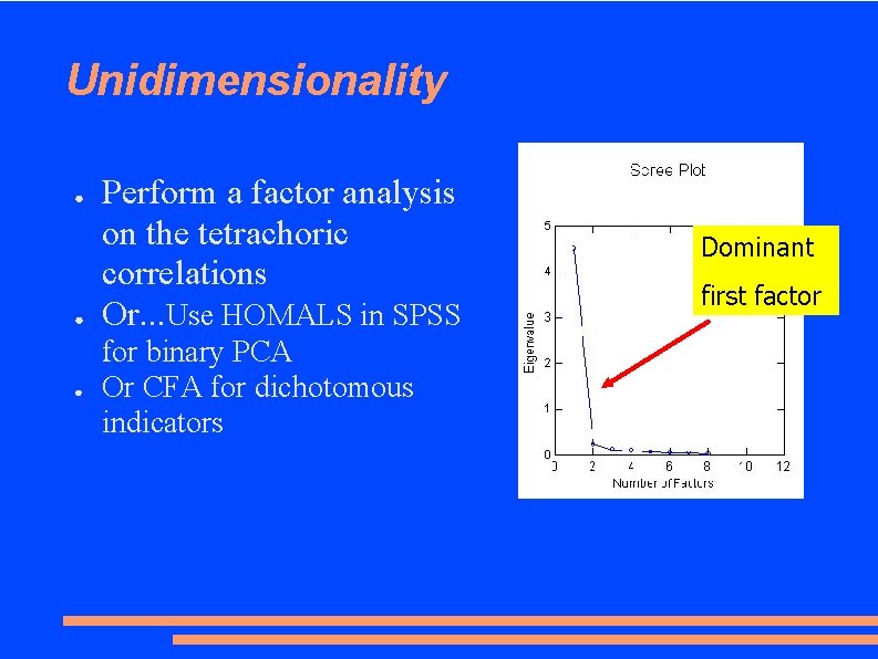
Unidimensionality ● ● ● Perform a factor analysis on the tetrachoric correlations Or. . . Use HOMALS in SPSS for binary PCA Or CFA for dichotomous indicators Dominant first factor

IRT vs. CTT ● Fan, X. (1998) Item Response Theory and Classical test Theory: an empirical comparison of their item/person statistics. Educational and Psychological Measurement, 58, 3, 357 -381. – There is no obvious superiority between classical sum-score item and test parameters and the new item response theory item and test parameters, when a large, representative sample of individuals are used to calibrate items.

Computer Adaptive Testing (CAT) ● ● ● In IRT, a person’s estimate of true score is not dependent upon the number of items correct Therefore, can use different items to measure different people and tailor a test to the individual Provides greater – – ● Efficiency (fewer items) Control of precision - given adequate items, every person can be measured with the same degree of precision Example: GRE

Components of a CAT system • A pre-calibrated bank of test items – Need to administer a large group of items to a large sample and estimate item parameters • An entry point into the item bank – i. e. , a rule for selecting the first item to be administered – Item difficulty, e. g. , b = 0, -3, or +3 – Use prior information about examinee

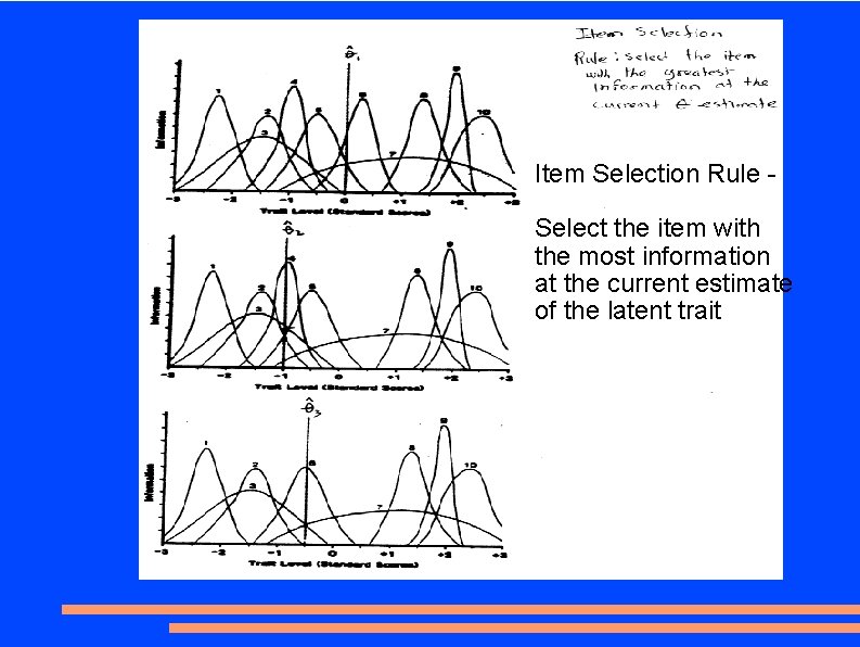
Components of a CAT system • An item selection or branching rule(s) – E. g. , if correct to first item, go to a more difficult item – If incorrect go to a less difficult item – Always select the most informative item at the current estimate of the trait level – As responses accumulate more information is gained about the examinee’s trait level

Item Selection Rule Select the item with the most information at the current estimate of the latent trait

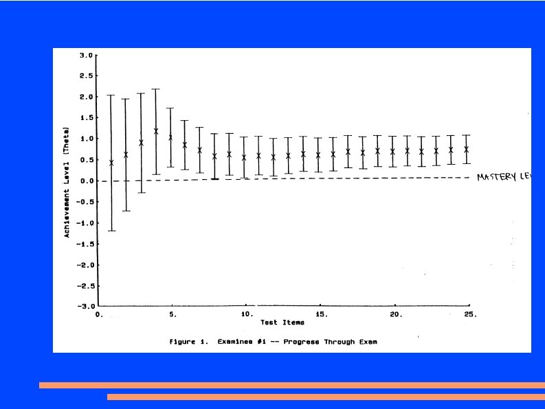
Components of a CAT system • A termination rule – Fixed number of items – Equiprecision ● ● – End when SEM around the examinee’s trait score has reached a certain level of precision The precision of test varies across individuals Examinee’s whose responses are consistent with the model will be easier to measure, i. e. , require fewer items Equiclassification ● SEM around trait estimate is above or below a cutoff level