MATHEMATICAL MODELING Why Modeling Fundamental and quantitative way

MATHEMATICAL MODELING

Why Modeling? Fundamental and quantitative way to understand analyze complex systems and phenomena. Complement to Theory and Experiments, and often integrate them. Becoming widespread in: Computational Physics, Chemistry, Mechanics, Materials, Biology, etc. 2

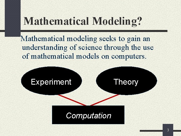
Mathematical Modeling? Mathematical modeling seeks to gain an understanding of science through the use of mathematical models on computers. Experiment Theory Computation 3

Mathematical Modeling Is often used in place of experiments when experiments are too large, too expensive, too dangerous, or too time consuming. Can be useful to investigate the use of pathogens (viruses, bacteria) to control an insect population, tumor growth, etc. Is a modern tool for scientific investigation. 4

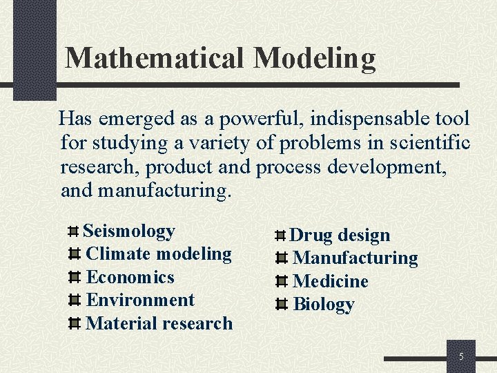
Mathematical Modeling Has emerged as a powerful, indispensable tool for studying a variety of problems in scientific research, product and process development, and manufacturing. Seismology Climate modeling Economics Environment Material research Drug design Manufacturing Medicine Biology 5

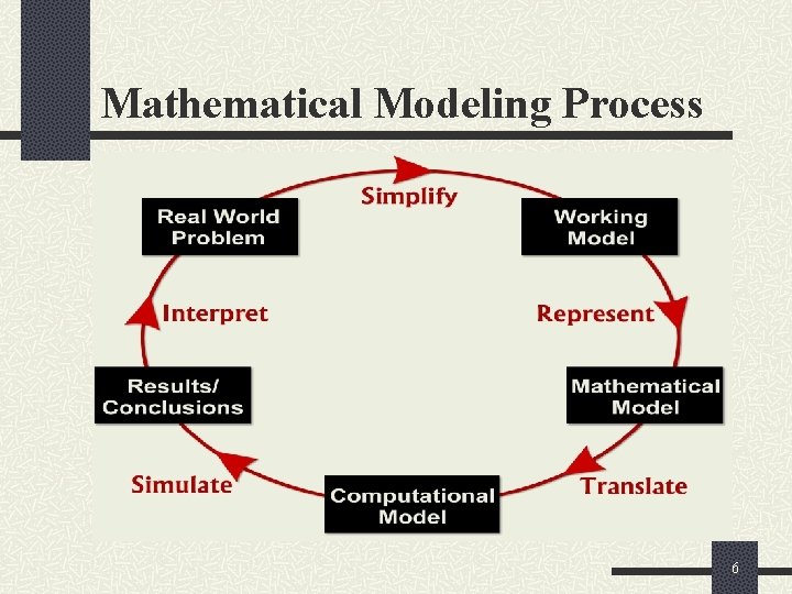
Mathematical Modeling Process 6

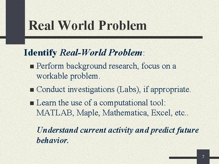
Real World Problem Identify Real-World Problem: n Perform background research, focus on a workable problem. n Conduct investigations (Labs), if appropriate. n Learn the use of a computational tool: MATLAB, Maple, Mathematica, Excel, etc. . Understand current activity and predict future behavior. 7

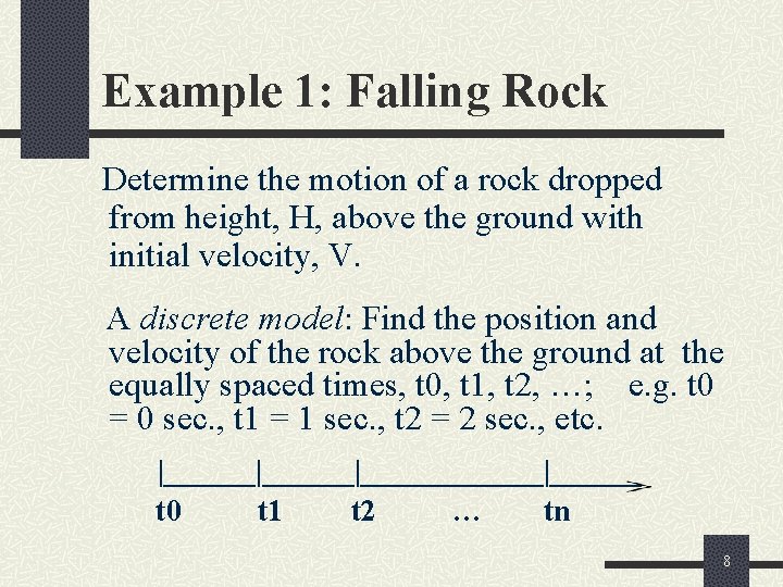
Example 1: Falling Rock Determine the motion of a rock dropped from height, H, above the ground with initial velocity, V. A discrete model: Find the position and velocity of the rock above the ground at the equally spaced times, t 0, t 1, t 2, …; e. g. t 0 = 0 sec. , t 1 = 1 sec. , t 2 = 2 sec. , etc. |______|______|______ t 0 t 1 t 2 … tn 8

Working Model Simplify Working Model: Identify and select factors to describe important aspects of Real World Problem; determine those factors that can be neglected. n State simplifying assumptions. n Determine governing principles, physical laws. n Identify model variables and inter-relationships. 9

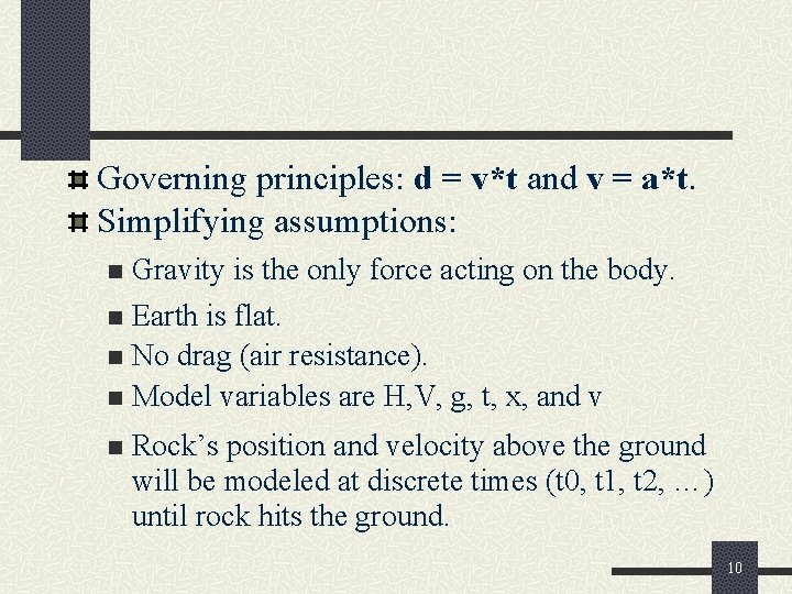
Governing principles: d = v*t and v = a*t. Simplifying assumptions: Gravity is the only force acting on the body. n Earth is flat. n No drag (air resistance). n Model variables are H, V, g, t, x, and v n n Rock’s position and velocity above the ground will be modeled at discrete times (t 0, t 1, t 2, …) until rock hits the ground. 10

Mathematical Model Represent Mathematical Model: Express the Working Model in mathematical terms; write down mathematical equations whose solution describes the Working Model. In general, the success of a mathematical model depends on how easy it is to use and how accurately it predicts. 11

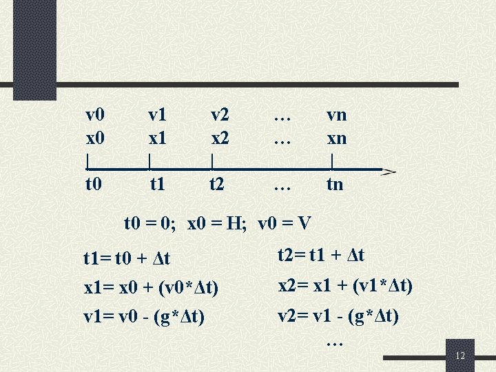
v 0 v 1 v 2 … vn x 0 x 1 x 2 … xn |______|______|_____ t 0 t 1 t 2 … tn t 0 = 0; x 0 = H; v 0 = V t 1= t 0 + Δt x 1= x 0 + (v 0*Δt) t 2= t 1 + Δt v 1= v 0 - (g*Δt) v 2= v 1 - (g*Δt) … x 2= x 1 + (v 1*Δt) 12

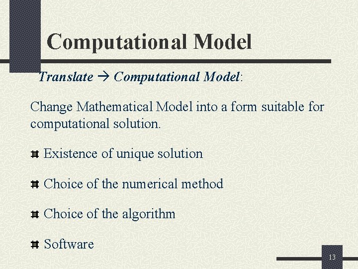
Computational Model Translate Computational Model: Change Mathematical Model into a form suitable for computational solution. Existence of unique solution Choice of the numerical method Choice of the algorithm Software 13

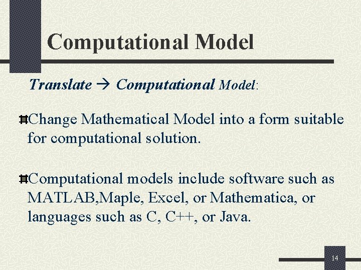
Computational Model Translate Computational Model: Change Mathematical Model into a form suitable for computational solution. Computational models include software such as MATLAB, Maple, Excel, or Mathematica, or languages such as C, C++, or Java. 14

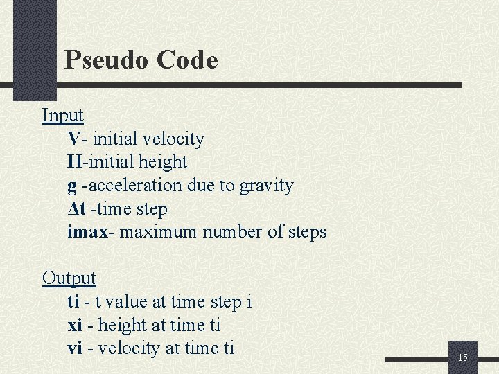
Pseudo Code Input V- initial velocity H-initial height g -acceleration due to gravity Δt -time step imax- maximum number of steps Output ti - t value at time step i xi - height at time ti vi - velocity at time ti 15

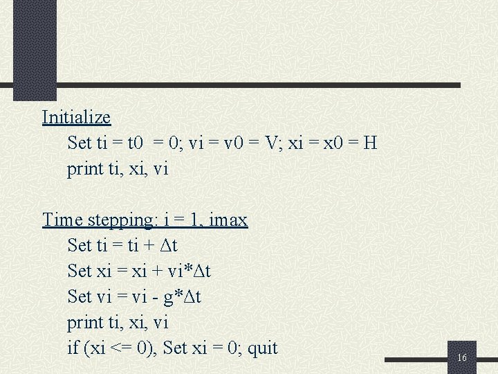
Initialize Set ti = t 0 = 0; vi = v 0 = V; xi = x 0 = H print ti, xi, vi Time stepping: i = 1, imax Set ti = ti + Δt Set xi = xi + vi*Δt Set vi = vi - g*Δt print ti, xi, vi if (xi <= 0), Set xi = 0; quit 16

Results/Conclusions Simulate Results/Conclusions: Run “Computational Model” to obtain Results; draw Conclusions. Verify your computer program; use check cases; explore ranges of validity. n Graphs, charts, and other visualization tools are useful in summarizing results and drawing conclusions. n 17

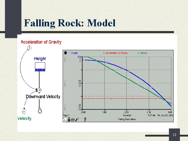
Falling Rock: Model 18

Interpret Conclusions If model results do not “agree” with physical reality or experimental data, reexamine the Working Model (assumptions) and repeat modeling steps. Often, the modeling process proceeds through several iterations until model is “acceptable”. 19

Interpret Conclusions(ctd. ) To create a more realistic model of a falling rock, some of the simplifying assumptions could be dropped; e. g. , incorporate drag - depends on shape of the rock is proportional to velocity. Improve discrete model: n Approximate velocities in the midpoint of time intervals instead of the beginning. n Reduce the size of Δt. 20

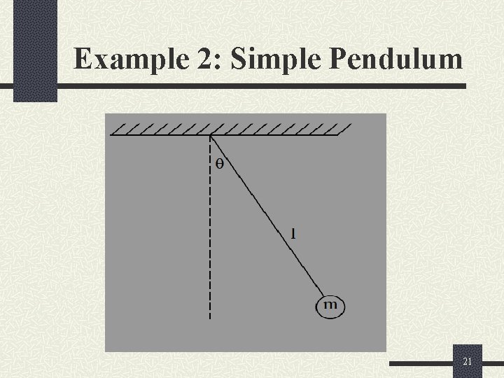
Example 2: Simple Pendulum 21

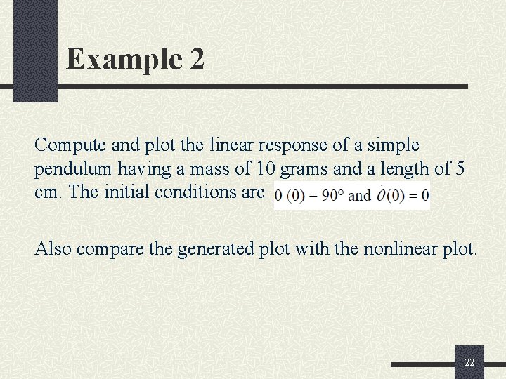
Example 2 Compute and plot the linear response of a simple pendulum having a mass of 10 grams and a length of 5 cm. The initial conditions are Also compare the generated plot with the nonlinear plot. 22

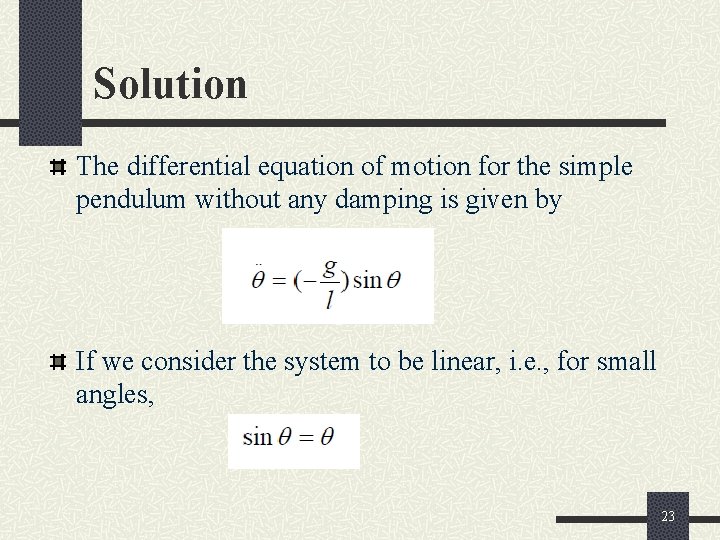
Solution The differential equation of motion for the simple pendulum without any damping is given by If we consider the system to be linear, i. e. , for small angles, 23

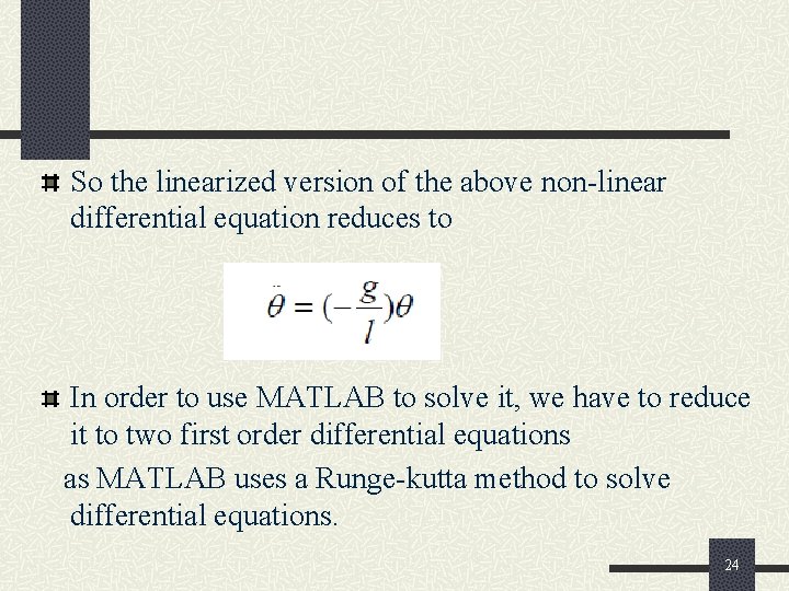
So the linearized version of the above non-linear differential equation reduces to In order to use MATLAB to solve it, we have to reduce it to two first order differential equations as MATLAB uses a Runge-kutta method to solve differential equations. 24

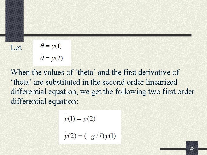
Let When the values of ‘theta’ and the first derivative of ‘theta’ are substituted in the second order linearized differential equation, we get the following two first order differential equation: 25

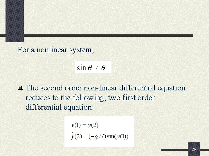
For a nonlinear system, The second order non-linear differential equation reduces to the following, two first order differential equation: 26

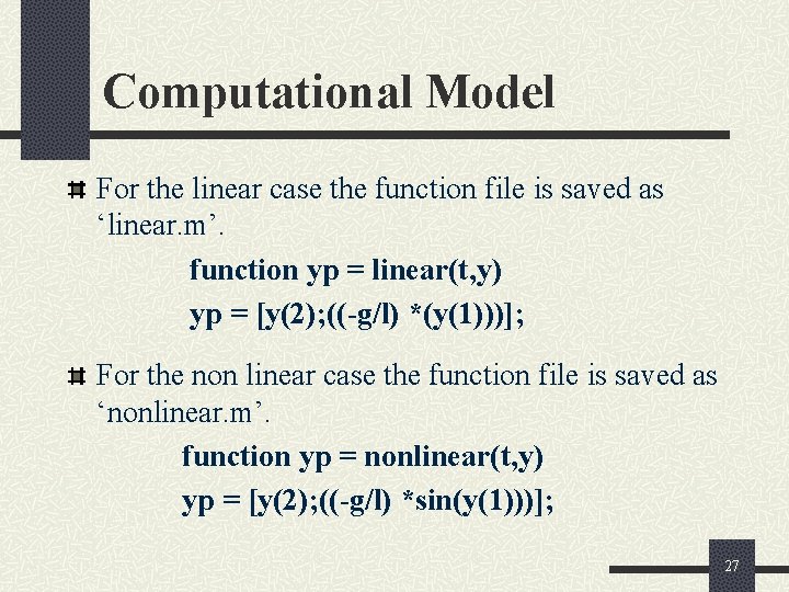
Computational Model For the linear case the function file is saved as ‘linear. m’. function yp = linear(t, y) yp = [y(2); ((-g/l) *(y(1)))]; For the non linear case the function file is saved as ‘nonlinear. m’. function yp = nonlinear(t, y) yp = [y(2); ((-g/l) *sin(y(1)))]; 27

Computational Model The main code should be written in a separate Mfile, which will actually call the above function files, solve the derivatives stored in them and plot the required result. ‘tspan’ represents the time interval and ‘y 0’ represents the initial condition. Note that the value of Ө in the initial conditions must be expressed in radians. 28

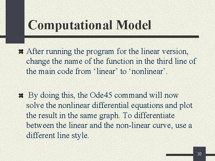
Computational Model tspan = [0 5]; y 0 = [1. 57; 0]; [t, y] = ode 45('linear', tspan, y 0) plot(t, y(: , 1)) grid on; xlabel(‘Time’) ylabel(‘Theta’) title(‘Theta Vs Time’) hold on; 29

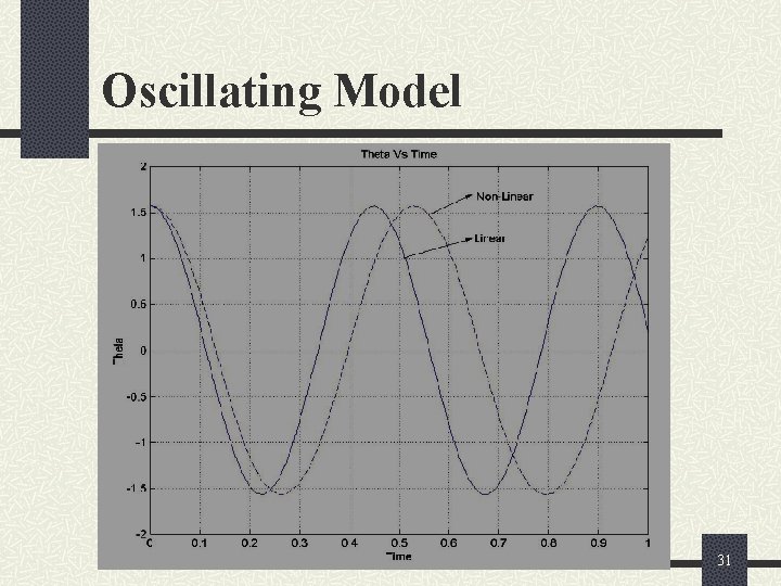
Computational Model After running the program for the linear version, change the name of the function in the third line of the main code from ‘linear’ to ‘nonlinear’. By doing this, the Ode 45 command will now solve the nonlinear differential equations and plot the result in the same graph. To differentiate between the linear and the non-linear curve, use a different line style. 30

Oscillating Model 31

Conclusions From the plots we can see that the time period for the non linear equation is greater than that of the linear equation. 32

Thank You! 33