Quantitative StructureActivity Relationships Quantitative StructurePropertyRelationships SARQSPR modeling Alexandre

Quantitative Structure-Activity Relationships Quantitative Structure-Property-Relationships SAR/QSPR modeling Alexandre Varnek Faculté de Chimie, ULP, Strasbourg, FRANCE

SAR/QSPR models • Development • Validation • Application

Classification and Regression models • Development • Validation • Application

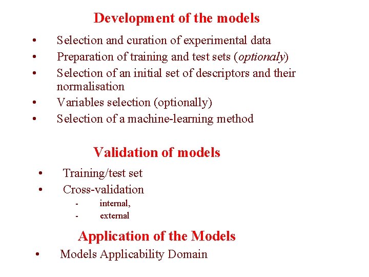
Development of the models • • • Selection and curation of experimental data Preparation of training and test sets (optionaly) Selection of an initial set of descriptors and their normalisation Variables selection (optionally) Selection of a machine-learning method • • Validation of models • • Training/test set Cross-validation - internal, external Application of the Models • Models Applicability Domain

Development the models • • Experimental Data: selection and cleaning Descriptors Mathematical techniques Statistical criteria

Data selection: Congenericity problem • Congenericity principle is the assumption that « similar compounds give similar responses » . This was the basic requirement of QSAR. This concerns structurally homogeneous data sets. • Nowdays, experimentalists mostly produce structurally diverse (non-congeneric) data sets

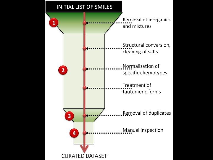
Data cleaning: • • • Similar experimental conditions Dublicates Structures standardization Removal of mixtures …. .

The importance of Chemical Data Curation Dataset curation is crucial for any cheminformatics analysis (QSAR modeling, clustering, similarity search, etc. ). Currently, it is uncommon to describe procedures used for curation in research papers; procedures are implemented or employed differently in different groups. We wish to emphasize the need to create and popularize standardized curation strategy, applicable for any ensemble of compounds.

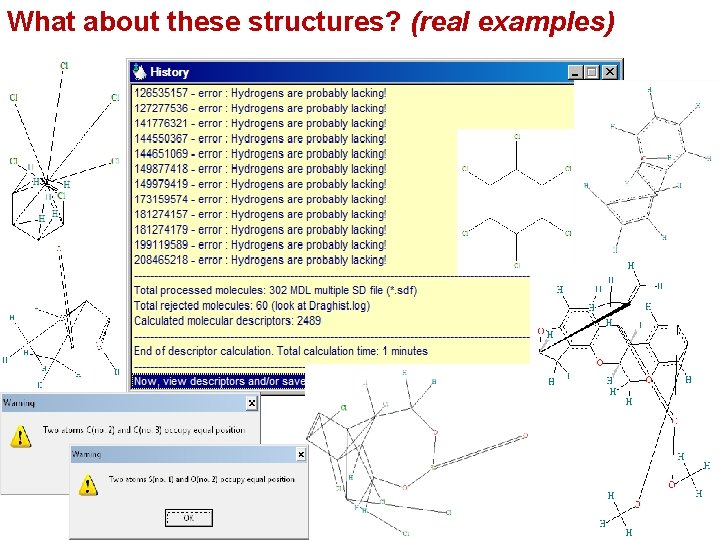
What about these structures? (real examples)

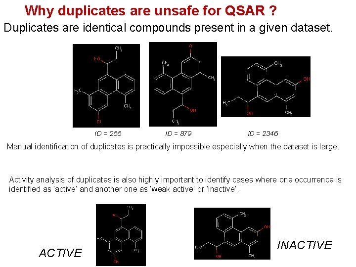
Why duplicates are unsafe for QSAR ? Duplicates are identical compounds present in a given dataset. ID = 256 ID = 879 ID = 2346 Manual identification of duplicates is practically impossible especially when the dataset is large. Activity analysis of duplicates is also highly important to identify cases where one occurrence is identified as ‘active’ and another one as ‘weak active’ or ‘inactive’. ACTIVE INACTIVE

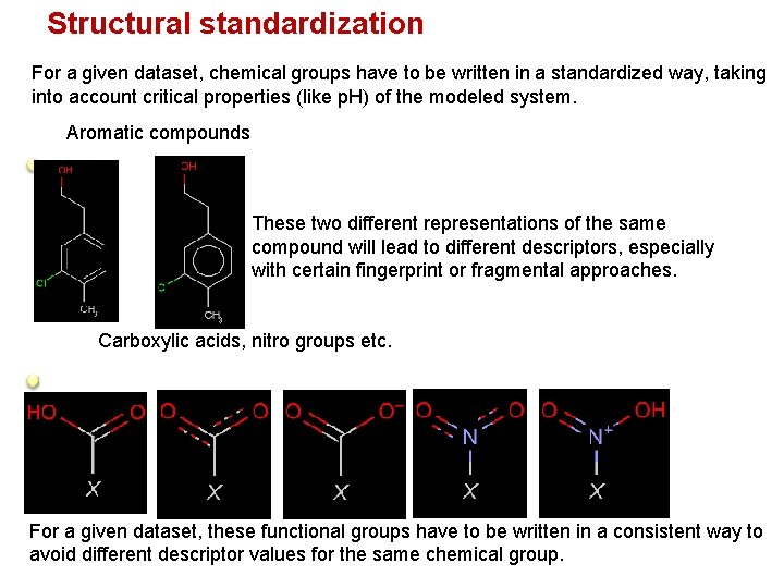
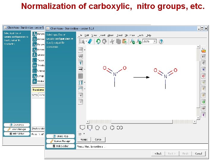
Structural standardization For a given dataset, chemical groups have to be written in a standardized way, taking into account critical properties (like p. H) of the modeled system. Aromatic compounds These two different representations of the same compound will lead to different descriptors, especially with certain fingerprint or fragmental approaches. Carboxylic acids, nitro groups etc. For a given dataset, these functional groups have to be written in a consistent way to avoid different descriptor values for the same chemical group.

Normalization of carboxylic, nitro groups, etc.

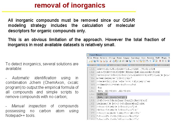
removal of inorganics All inorganic compounds must be removed since our QSAR modeling strategy includes the calculation of molecular descriptors for organic compounds only. This is an obvious limitation of the approach. However the total fraction of inorganics in most available datasets is relatively small. To detect inorganics, several solutions are available: - Automatic identification using in combination Jchem (Chem. Axon, cxcalc program) to output the empirical formula of all compounds and simple scripts to remove compounds with no carbon; - Manual inspection of compounds possessing no carbon atom using Notepad++ tools.

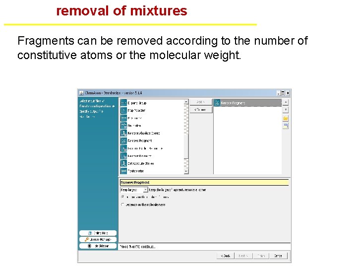
removal of mixtures Fragments can be removed according to the number of constitutive atoms or the molecular weight.

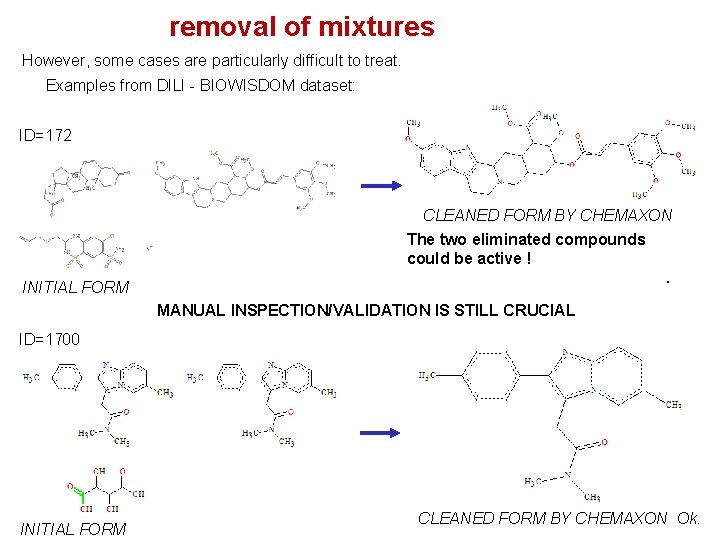
removal of mixtures However, some cases are particularly difficult to treat. Examples from DILI - BIOWISDOM dataset: ID=172 CLEANED FORM BY CHEMAXON The two eliminated compounds could be active !. INITIAL FORM MANUAL INSPECTION/VALIDATION IS STILL CRUCIAL ID=1700 INITIAL FORM CLEANED FORM BY CHEMAXON Ok.

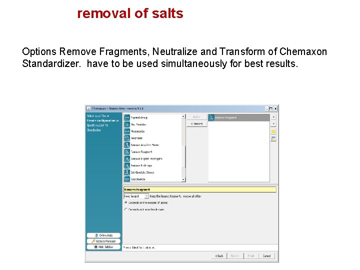
removal of salts Options Remove Fragments, Neutralize and Transform of Chemaxon Standardizer. have to be used simultaneously for best results.

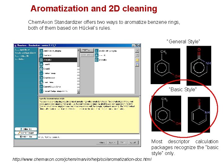
Aromatization and 2 D cleaning Chem. Axon Standardizer offers two ways to aromatize benzene rings, both of them based on Hűckel’s rules. “General Style” “Basic Style” Most descriptor calculation packages recognize the “basic style” only. http: //www. chemaxon. com/jchem/marvin/help/sci/aromatization-doc. html

Preparation of training and test sets Building of structure property models Training set Initial data set Test 10 – 15 % Splitting of an initial data set into training and test sets Selection of the best models according to statistical criteria “Prediction” calculations using the best structure property models

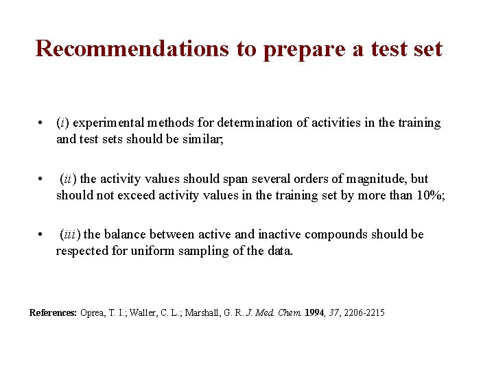
Recommendations to prepare a test set • (i) experimental methods for determination of activities in the training and test sets should be similar; • (ii) the activity values should span several orders of magnitude, but should not exceed activity values in the training set by more than 10%; • (iii) the balance between active and inactive compounds should be respected for uniform sampling of the data. References: Oprea, T. I. ; Waller, C. L. ; Marshall, G. R. J. Med. Chem. 1994, 37, 2206 -2215

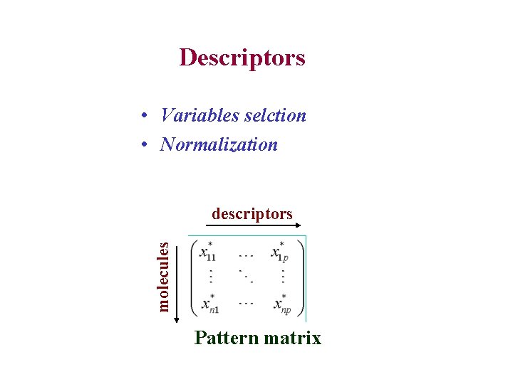
Descriptors • Variables selction • Normalization molecules descriptors Pattern matrix

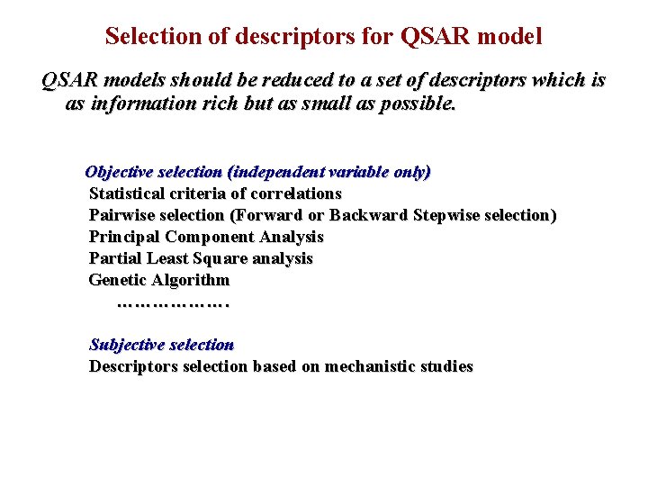
Selection of descriptors for QSAR models should be reduced to a set of descriptors which is as information rich but as small as possible. Objective selection (independent variable only) Statistical criteria of correlations Pairwise selection (Forward or Backward Stepwise selection) Principal Component Analysis Partial Least Square analysis Genetic Algorithm ………………. Subjective selection Descriptors selection based on mechanistic studies

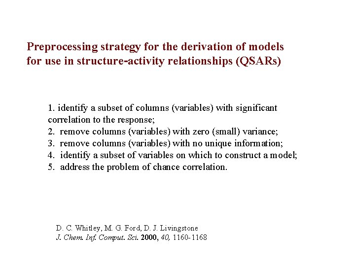
Preprocessing strategy for the derivation of models for use in structure-activity relationships (QSARs) 1. identify a subset of columns (variables) with significant correlation to the response; 2. remove columns (variables) with zero (small) variance; 3. remove columns (variables) with no unique information; 4. identify a subset of variables on which to construct a model; 5. address the problem of chance correlation. D. C. Whitley, M. G. Ford, D. J. Livingstone J. Chem. Inf. Comput. Sci. 2000, 40, 1160 -1168

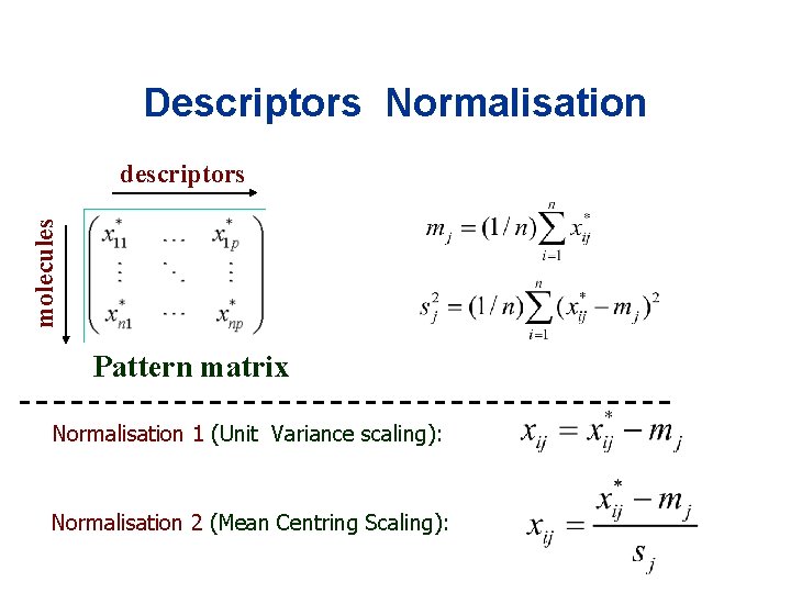
Descriptors Normalisation molecules descriptors Pattern matrix Normalisation 1 (Unit Variance scaling): Normalisation 2 (Mean Centring Scaling):

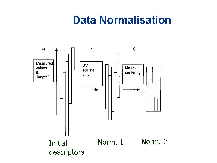
Data Normalisation Initial descriptors Norm. 1 Norm. 2

Machine-Learning Methods

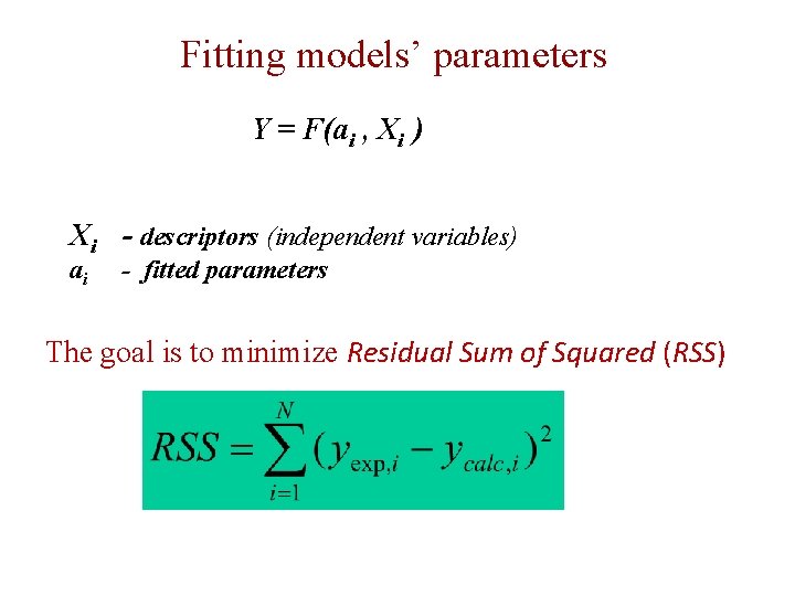
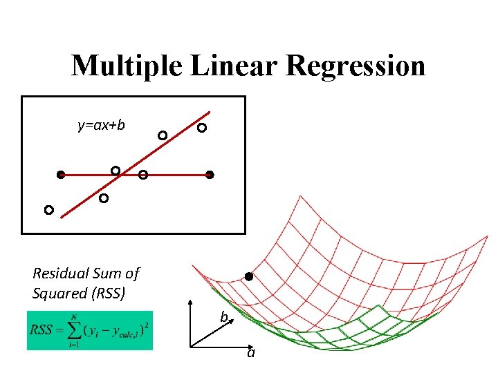
Fitting models’ parameters Y = F(ai , Xi ) Xi - descriptors (independent variables) ai - fitted parameters The goal is to minimize Residual Sum of Squared (RSS)

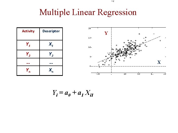
Multiple Linear Regression Activity Descriptor Y 1 X 1 Y 2 … … Yn Xn Yi = a 0 + a 1 Xi 1 Y X

Multiple Linear Regression y=ax+b Residual Sum of Squared (RSS) b a

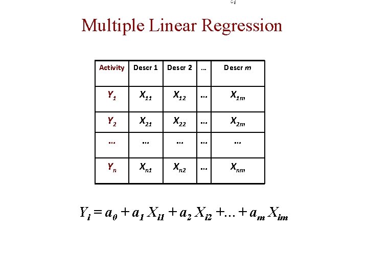
Multiple Linear Regression Activity Descr 1 Descr 2 … Descr m Y 1 X 12 … X 1 m Y 2 X 21 X 22 … X 2 m … … … Yn Xn 1 Xn 2 … Xnm Yi = a 0 + a 1 Xi 1 + a 2 Xi 2 +…+ am Xim

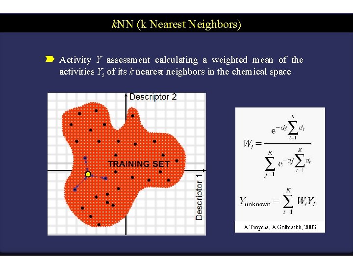
k. NN (k Nearest Neighbors) Activity Y assessment calculating a weighted mean of the activities Yi of its k nearest neighbors in the chemical space TRAINING SET Descriptor 1 Descriptor 2 A. Tropsha, A. Golbraikh, 2003

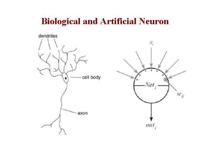
Biological and Artificial Neuron

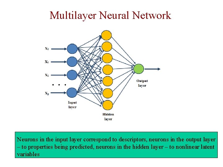
Multilayer Neural Network Neurons in the input layer correspond to descriptors, neurons in the output layer – to properties being predicted, neurons in the hidden layer – to nonlinear latent variables

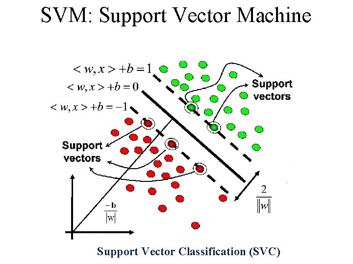
SVM: Support Vector Machine Support Vector Classification (SVC)

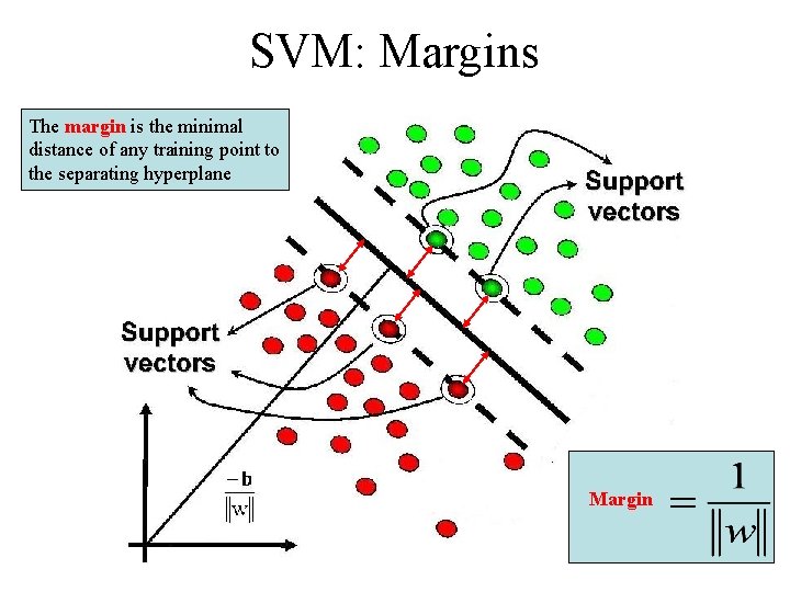
SVM: Margins The margin is the minimal distance of any training point to the separating hyperplane Margin

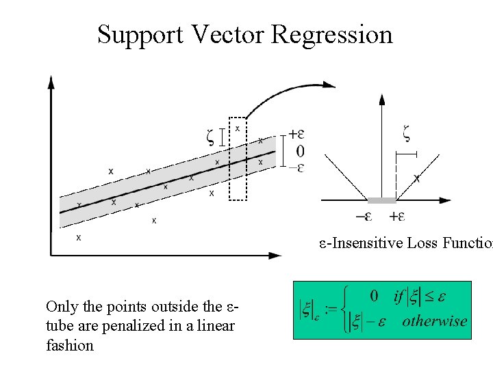
Support Vector Regression ε-Insensitive Loss Function Only the points outside the εtube are penalized in a linear fashion

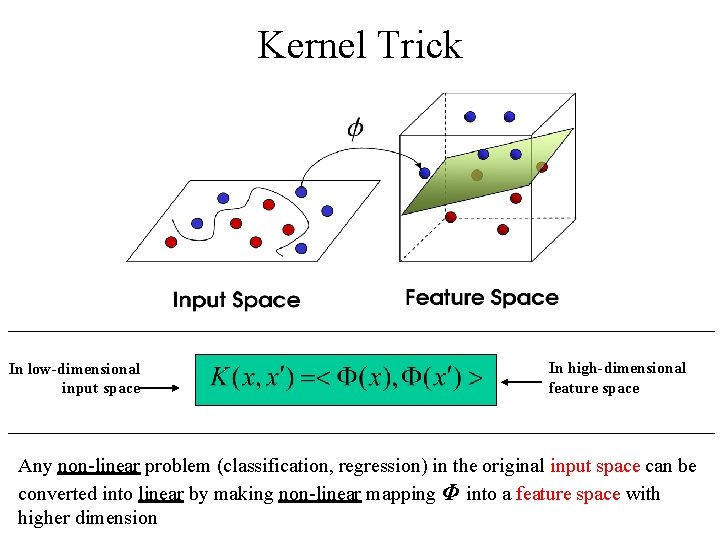
Kernel Trick In low-dimensional input space In high-dimensional feature space Any non-linear problem (classification, regression) in the original input space can be converted into linear by making non-linear mapping Φ into a feature space with higher dimension

QSAR/QSPR models • Development • Validation • Application

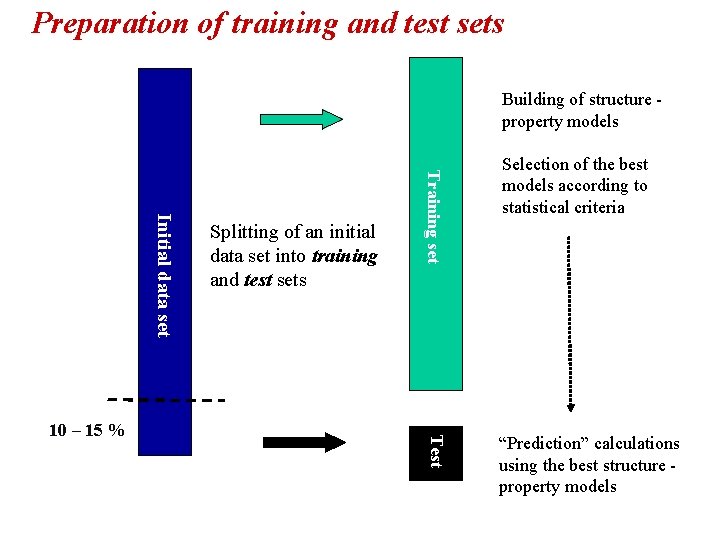
Preparation of training and test sets Building of structure property models Training set Initial data set Test 10 – 15 % Splitting of an initial data set into training and test sets Selection of the best models according to statistical criteria “Prediction” calculations using the best structure property models

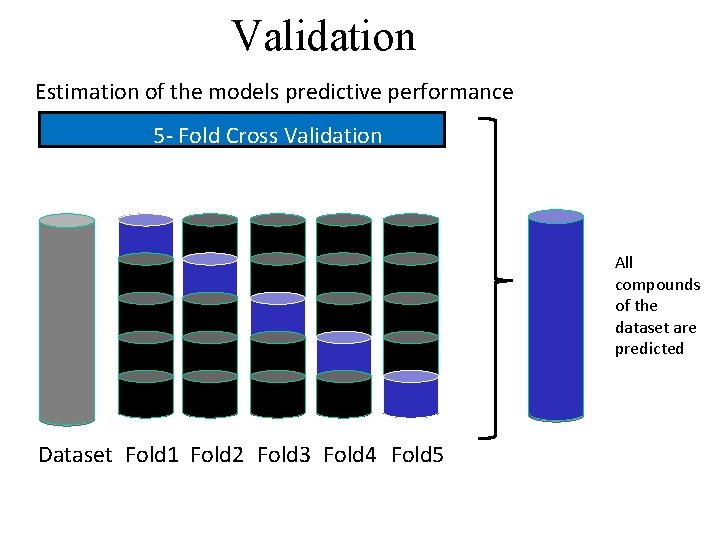
Validation Estimation of the models predictive performance 5 - Fold Cross Validation All compounds of the dataset are predicted Dataset Fold 1 Fold 2 Fold 3 Fold 4 Fold 5

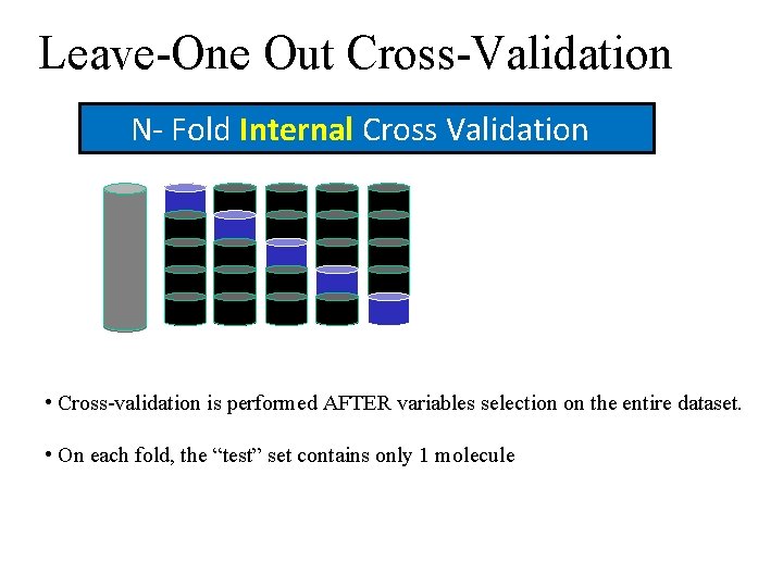
Leave-One Out Cross-Validation N- Fold Internal Cross Validation • Cross-validation is performed AFTER variables selection on the entire dataset. • On each fold, the “test” set contains only 1 molecule

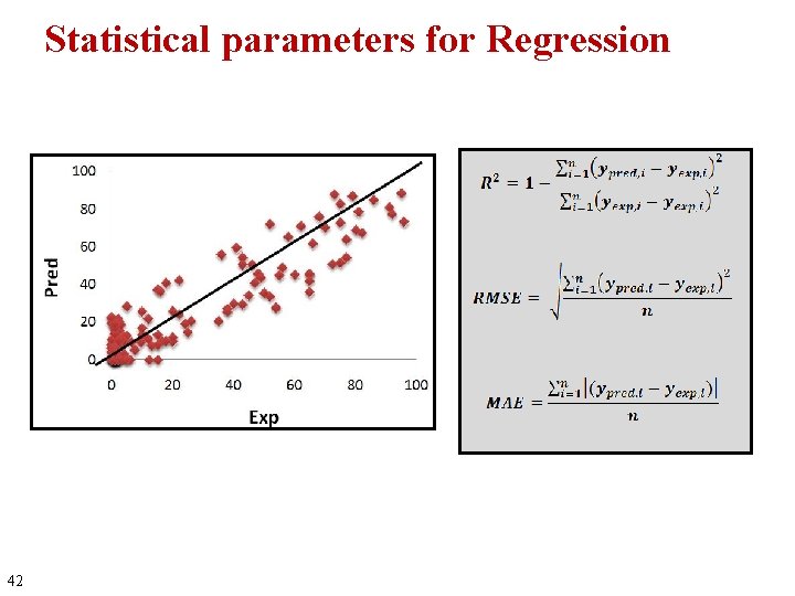
Statistical parameters for Regression 42

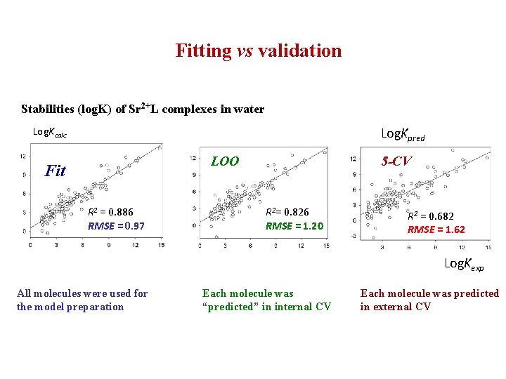
Fitting vs validation Stabilities (log. K) of Sr 2+L complexes in water Log. Kpred Log. Kcalc LOO Fit R 2 = 0. 886 RMSE = 0. 97 5 -CV R 2= 0. 826 RMSE = 1. 20 R 2 = 0. 682 RMSE = 1. 62 Log. Kexp All molecules were used for the model preparation Each molecule was “predicted” in internal CV Each molecule was predicted in external CV

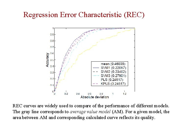
Regression Error Characteristic (REC) REC curves are widely used to compare of the performance of different models. The gray line corresponds to average value model (AM). For a given model, the area between AM and corresponding calculated curve reflects its quality.

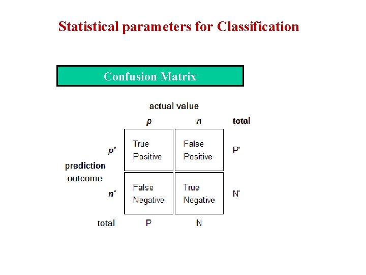
Statistical parameters for Classification Confusion Matrix

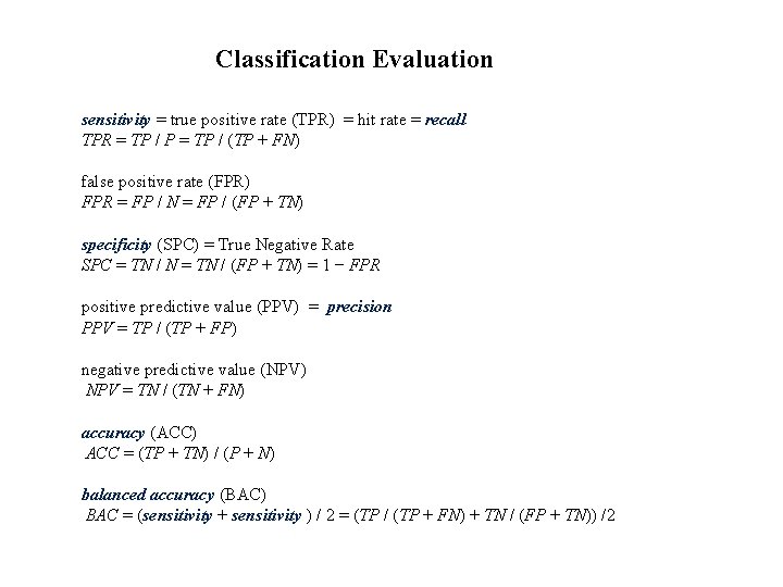
Classification Evaluation sensitivity = true positive rate (TPR) = hit rate = recall TPR = TP / P = TP / (TP + FN) false positive rate (FPR) FPR = FP / N = FP / (FP + TN) specificity (SPC) = True Negative Rate SPC = TN / N = TN / (FP + TN) = 1 − FPR positive predictive value (PPV) = precision PPV = TP / (TP + FP) negative predictive value (NPV) NPV = TN / (TN + FN) accuracy (ACC) ACC = (TP + TN) / (P + N) balanced accuracy (BAC) BAC = (sensitivity + sensitivity ) / 2 = (TP / (TP + FN) + TN / (FP + TN)) /2

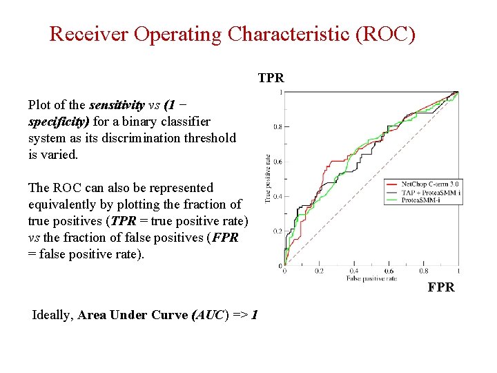
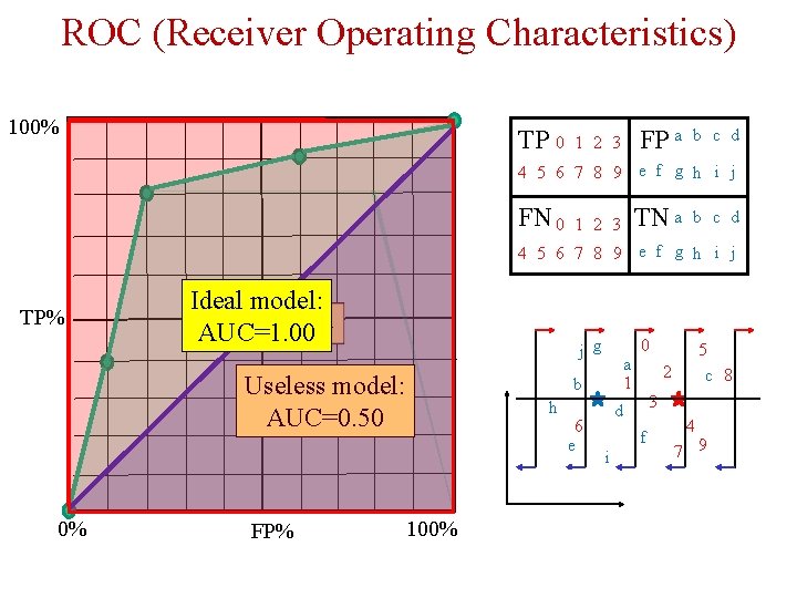
Receiver Operating Characteristic (ROC) TPR Plot of the sensitivity vs (1 − specificity) for a binary classifier system as its discrimination threshold is varied. The ROC can also be represented equivalently by plotting the fraction of true positives (TPR = true positive rate) vs the fraction of false positives (FPR = false positive rate). FPR Ideally, Area Under Curve (AUC) => 1

ROC (Receiver Operating Characteristics) 100% TP 0 FP a 1 2 3 b c d 4 5 6 7 8 9 e f g h i j FN 0 TN a 1 2 3 b c d 4 5 6 7 8 9 e f g h i j TP% Ideal model: AUC=0. 84 AUC=1. 00 j g Useless model: AUC=0. 50 0% FP% a 1 b h 100% 6 e 0 2 3 d f i 5 c 8 4 7 9

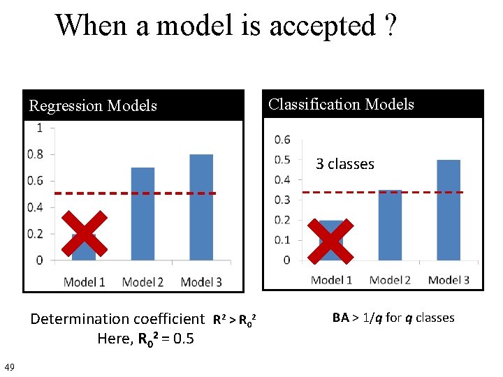
When a model is accepted ? Regression Models Classification Models 3 classes Determination coefficient R 2 > R 02 Here, R 02 = 0. 5 49 BA > 1/q for q classes

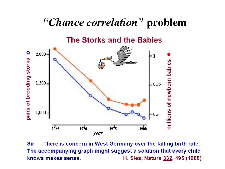
“Chance correlation” problem 2, 000 1 1, 500 0. 75 1, 000 0. 5 1965 1970 year 1975 1980

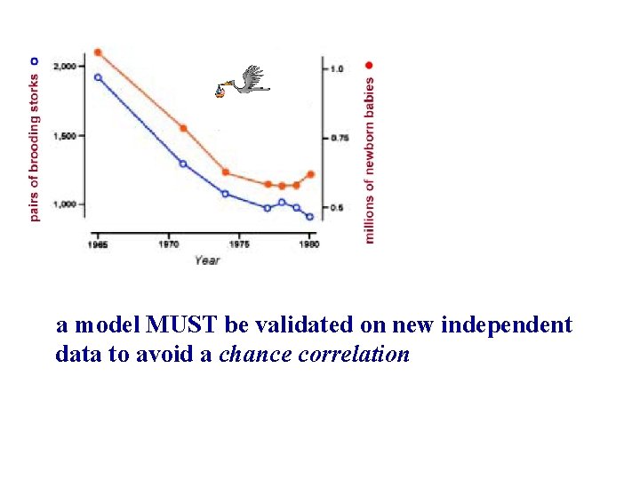
a model MUST be validated on new independent data to avoid a chance correlation

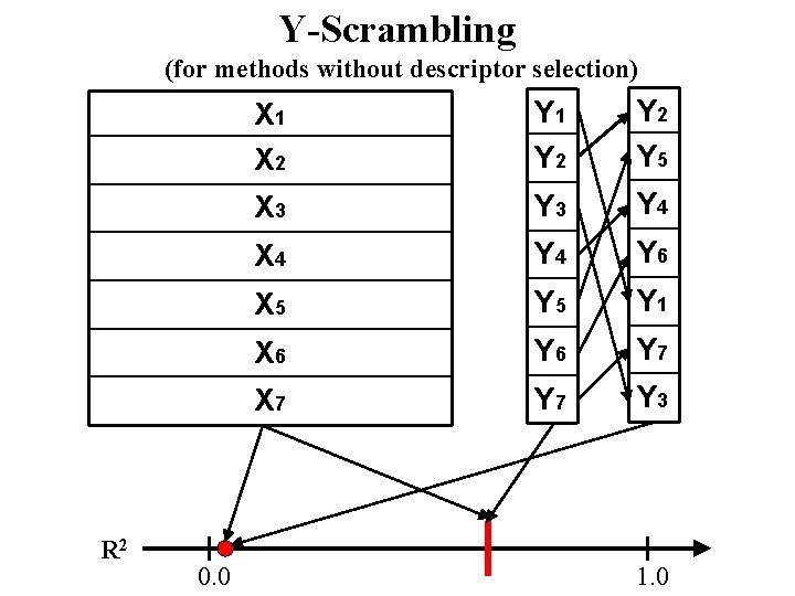
Y-Scrambling (for methods without descriptor selection) R 2 0. 0 X 1 X 2 Y 1 Y 2 Y 5 X 3 Y 4 X 4 Y 6 X 5 Y 1 X 6 Y 7 X 7 Y 3 1. 0

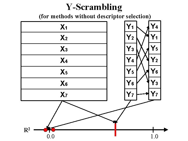
Y-Scrambling (for methods without descriptor selection) R 2 0. 0 X 1 X 2 Y 1 Y 2 Y 4 Y 1 X 3 Y 5 X 4 Y 2 X 5 Y 6 X 6 Y 3 X 7 Y 7 1. 0

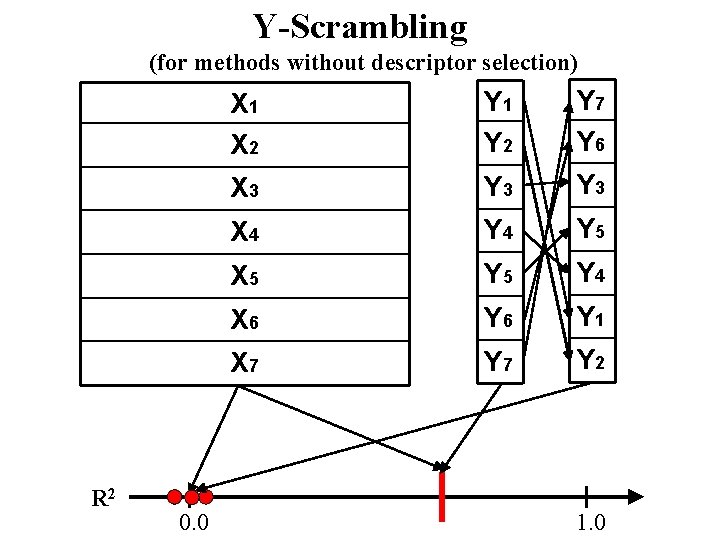
Y-Scrambling (for methods without descriptor selection) R 2 0. 0 X 1 X 2 Y 1 Y 2 Y 7 Y 6 X 3 Y 3 X 4 Y 5 X 5 Y 4 X 6 Y 1 X 7 Y 2 1. 0

QSAR/QSPR models • Development • Validation • Application

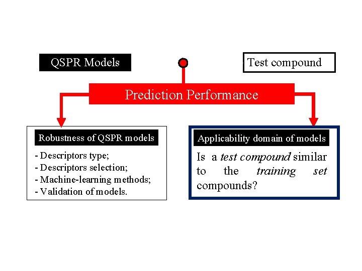
Test compound QSPR Models Prediction Performance Robustness of QSPR models - Descriptors type; - Descriptors selection; - Machine-learning methods; - Validation of models. Applicability domain of models Is a test compound similar to the training set compounds?

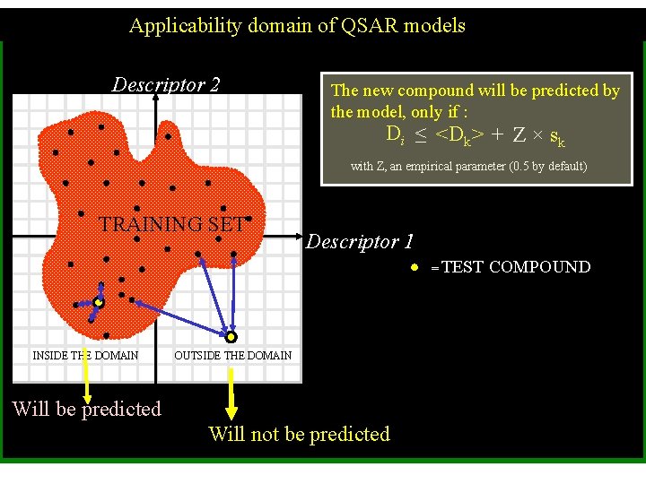
Applicability domain of QSAR models Descriptor 2 The new compound will be predicted by the model, only if : Di ≤ <Dk> + Z × sk with Z, an empirical parameter (0. 5 by default) TRAINING SET Descriptor 1 = TEST INSIDE THE DOMAIN OUTSIDE THE DOMAIN Will be predicted Will not be predicted COMPOUND

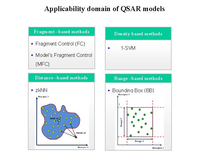
domain of QSAR models Applicability Domain Approaches Fragment –based methods § Fragment Control (FC) Density based methods § 1 -SVM § Model’s Fragment Control (MFC) Distance –based methods § zk. NN Range –based methods § Bounding Box (BB)

Ensemble modeling

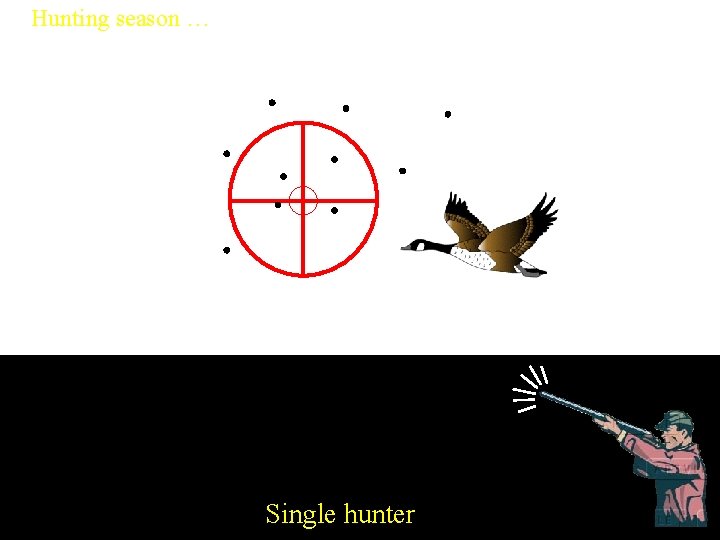
Hunting season … Single hunter

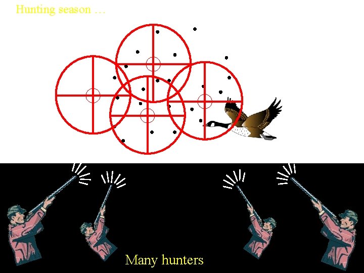
Hunting season … Many hunters

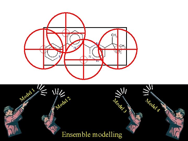
el d o 1 2 el od o M l de M M 3 Ensemble modelling M od el 4

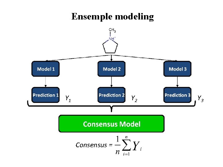
Ensemple modeling Y 1 Y 2 Consensus = Y 3

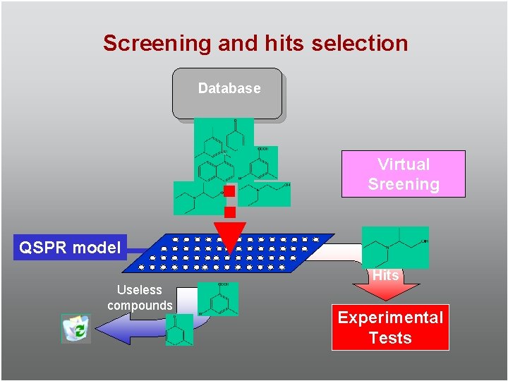
Screening and hits selection Database Virtual Sreening QSPR model Useless compounds Hits Experimental Tests