Math 5364 Notes Chapter 4 Classification Jesse Crawford


 No N =")
 Refund N =")
 Refund N =")
 Refund N =")


 No N =")
 Refund Yes No")
 Refund Yes No")
 Refund Yes No")


![Iris Data Set plot(Petal. Length, Petal. Width, col=c('blue', 'red', 'purple')[Species])](https://slidetodoc.com/presentation_image_h/78f2f661774e2be94628e76cec4bfca8/image-27.jpg "Iris Data Set plot(Petal. Length, Petal. Width, col=c('blue', 'red', 'purple')[Species])")
 library(rattle) iristree=rpart(Species~Sepal. Length+Sepal. Width+Petal. Length+Petal. Width, data=iris) iristree=rpart(Species~. , data=iris)")
 confusionmatrix=table(Species, pred. Species) confusionmatrix")
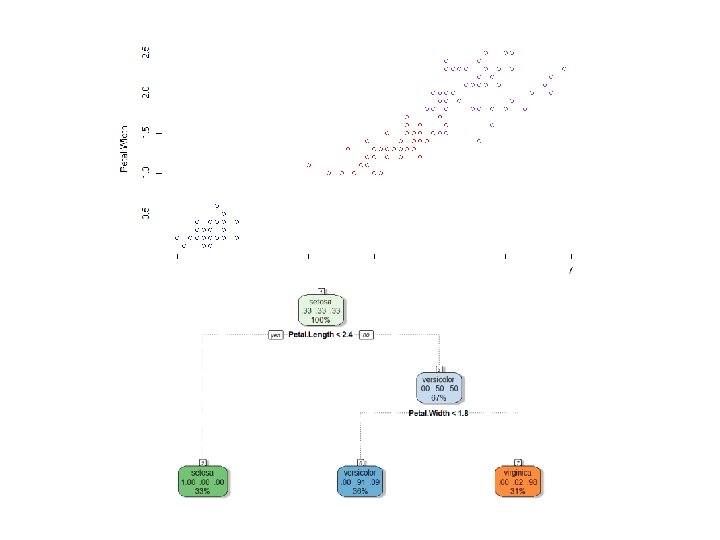
![plot(jitter(Petal. Length), jitter(Petal. Width), col=c('blue', 'red', 'purple')[Species]) lines(1: 7, rep(1. 8, 7), col='black') lines(rep(2.](https://slidetodoc.com/presentation_image_h/78f2f661774e2be94628e76cec4bfca8/image-31.jpg "plot(jitter(Petal. Length), jitter(Petal. Width), col=c('blue', 'red', 'purple')[Species]) lines(1: 7, rep(1. 8, 7), col='black') lines(rep(2.")
 confusionmatrix=table(Species, pred. Species) confusionmatrix")

)/sum(confusionmatrix) The accuracy is 96% Error rate is 4%")
 iristree 2=ctree(Species~. , data=iris) plot(iristree 2)")
")
 confusionmatrix=table(Species, pred. Species) confusionmatrix")
) plot(iristree 3)")


 fancy. Rpart. Plot(extree)")

) Training error = 36% Testing error = 39% 3")
) Training error = 30% Testing error = 34% 5")
) Training error = 28% Testing error = 34% 9")
) Training error = 24% Testing error = 30% 21")
) Training error = 21% Testing error = 29% 27")
) Default value of cp is 0. 01")
) Default value of cp is 0. 01")
) Default value of cp is 0. 01")
) Default value of cp is 0. 01 Lower")


 (0. 6891, 0. 7280)")
 (0. 6886, 0. 7279)")

 Use the mcnemar. exact function")


- Slides: 68
Math 5364 Notes Chapter 4: Classification Jesse Crawford Department of Mathematics Tarleton State University
Today's Topics • Preliminaries • Decision Trees • Hunt's Algorithm • Impurity measures
Preliminaries • Data: Table with rows and columns • Rows: People or objects being studied • Columns: Characteristics of those objects • Rows: Objects, subjects, records, cases, observations, sample elements. • Columns: Characteristics, attributes, variables, features
• Dependent variable Y: Variable being predicted. • Independent variables Xj : Variables used to make predictions. • Dependent variable: Response or output variable. • Independent variables: Predictors, explanatory variables, control variables, covariates, or input variables.
• Nominal variable: Values are names or categories with no ordinal structure. • Examples: Eye color, gender, refund, marital status, tax fraud. • Ordinal variable: Values are names or categories with an ordinal structure. • Examples: T-shirt size (small, medium, large) or grade in a class (A, B, C, D, F). • Binary/Dichotomous variable: Only two possible values. • Examples: Refund and tax fraud. • Categorical/qualitative variable: Term that includes all nominal and ordinal variables. • Quantitative variable: Variable with numerical values for which meaningful arithmetic operations can be applied. • Examples: Blood pressure, cholesterol, taxable income.
• Regression: Determining or predicting the value of a quantitative variable using other variables. • Classification: Determining or predicting the value of a categorical variable using other variables. • Classifying tumors as benign or malignant. • Classifying credit card transactions as legitimate or fraudulent. • Classifying secondary structures of protein as alpha-helix, beta-sheet, or random coil. • Classifying a user of a website as a real person or a bot. • Predicting whether a student will be retained/academically successful at a university.
• Related fields: Data mining/data science, machine learning, artificial intelligence, and statistics. • Classification learning algorithms: • Decision trees • Rule-based classifiers • Nearest-neighbor classifiers • Bayesian classifiers • Artificial neural networks • Support vector machines
Decision Trees Training Data Name Human Python Salmon Body Temperature Warm-blooded Cold-blooded Skin Cover hair scales Gives Birth yes no no Aquatic Creature no no yes Has Legs yes no no Class Label mammal non-mammal yes no yes semi no yes mammal non-mammal Whale Penguin Warm-blooded hair feathers Body Temperature Cold-blooded Warm-blooded Gives Birth? Non-mammal Yes No Mammal Non-mammal
Body Temperature Cold-blooded Warm-blooded Gives Birth? • • Non-mammal Yes No Mammal Non-mammal Chicken Classified as non-mammal Dog Classified as mammal Frog Classified as non-mammal Duck-billed platypus Classified as non-mammal (mistake)
Refund Yes No NO Mar. St Single, Divorced Tax. Inc < 80 K NO Married NO > 80 K YES
Hunt’s Algorithm (Basis of ID 3, C 4. 5, and CART) No N = 10 (7, 3)
Hunt’s Algorithm (Basis of ID 3, C 4. 5, and CART) Refund N = 10 (7, 3) Yes No NO NO N = 3 (3, 0) N = 7 (4, 3)
Hunt’s Algorithm (Basis of ID 3, C 4. 5, and CART) Refund N = 10 (7, 3) Yes No NO Mar. St N = 3 (3, 0) Single Divorced YES N = 4 (1, 3) N = 7 (4, 3) Married NO N = 3 (3, 0)
Hunt’s Algorithm (Basis of ID 3, C 4. 5, and CART) Refund N = 10 (7, 3) Yes No NO Mar. St N = 3 (3, 0) Married Single Divorced NO Tax. Inc < 80 K N = 7 (4, 3) > 80 K NO YES N = 1 (1, 0) N = 3 (0, 3) N = 3 (3, 0)
Impurity Measures No
Impurity Measures
Impurity Measures
Hunt’s Algorithm (Basis of ID 3, C 4. 5, and CART) No N = 10 (7, 3)
Hunt’s Algorithm (Basis of ID 3, C 4. 5, and CART) Refund Yes No NO NO N = 3 (3, 0) N = 7 (4, 3)
Hunt’s Algorithm (Basis of ID 3, C 4. 5, and CART) Refund Yes No NO Mar. St N = 3 (3, 0) Single Divorced YES N = 4 (1, 3) Married NO N = 3 (3, 0)
Hunt’s Algorithm (Basis of ID 3, C 4. 5, and CART) Refund Yes No NO Mar. St N = 3 (3, 0) Married Single Divorced NO Tax. Inc < 80 K > 80 K NO YES N = 1 (1, 0) N = 3 (0, 3) N = 3 (3, 0)
Types of Splits • Binary Split Single, Divorced Marital Status Married • Multi-way Split Marital Status Single Divorced Married
Types of Splits
Hunt’s Algorithm Details • Which variable should be used to split first? • Answer: the one that decreases impurity the most. • How should each variable be split? • Answer: in the manner that minimizes the impurity measure. • Stopping conditions: • If all records in a node have the same class label, it becomes a terminal node with that class label. • If all records in a node have the same attributes, it becomes a terminal node with label determined by majority rule. • If gain in impurity falls below a given threshold. • If tree reaches a given depth. • If other prespecified conditions are met.
Today's Topics • Data sets included in R • Decision trees with rpart and party packages • Using a tree to classify new data • Confusion matrices • Classification accuracy
Iris Data Set • Iris Flowers • 3 Species: Setosa, Versicolor, and Virginica • Variables: Sepal. Length, Sepal. Width, Petal. Length, and Petal. Width head(iris) attach(iris) plot(Petal. Length, Petal. Width, col=Species) plot(Petal. Length, Petal. Width, col=c('blue', 'red', 'purple')[Species])
Iris Data Set plot(Petal. Length, Petal. Width, col=c('blue', 'red', 'purple')[Species])
The rpart Package library(rpart) library(rattle) iristree=rpart(Species~Sepal. Length+Sepal. Width+Petal. Length+Petal. Width, data=iris) iristree=rpart(Species~. , data=iris) fancy. Rpart. Plot(iristree)
pred. Species=predict(iristree, newdata=iris, type="class") confusionmatrix=table(Species, pred. Species) confusionmatrix
plot(jitter(Petal. Length), jitter(Petal. Width), col=c('blue', 'red', 'purple')[Species]) lines(1: 7, rep(1. 8, 7), col='black') lines(rep(2. 4, 4), 0: 3, col='black')
pred. Species=predict(iristree, newdata=iris, type="class") confusionmatrix=table(Species, pred. Species) confusionmatrix
Predicted Class = 1 Class = 0 Class = 1 f 10 Class = 0 f 01 f 00 Confusion Matrix Actual Class
Accuracy for Iris Decision Tree accuracy=sum(diag(confusionmatrix))/sum(confusionmatrix) The accuracy is 96% Error rate is 4%
The party Package library(party) iristree 2=ctree(Species~. , data=iris) plot(iristree 2)
The party Package plot(iristree 2, type='simple')
Predictions with ctree pred. Species=predict(iristree 2, newdata=iris) confusionmatrix=table(Species, pred. Species) confusionmatrix
iristree 3=ctree(Species~. , data=iris, controls=ctree_control(maxdepth=2)) plot(iristree 3)
Today's Topics • Training and Test Data • Training error, test error, and generalization error • Underfitting and Overfitting • Confidence intervals and hypothesis tests for classification accuracy
Training and Testing Sets
Training and Testing Sets • Divide data into training data and test data. • Training data: used to construct classifier/statisical model • Test data: used to test classifier/model • Types of errors: • Training error rate: error rate on training data • Generalization error rate: error rate on all nontraining data • Test error rate: error rate on test data • Generalization error is most important • Use test error to estimate generalization error • Entire process is called cross-validation
Example Data
Split 30% training data and 70% test data. extree=rpart(class~. , data=traindata) fancy. Rpart. Plot(extree) plot(extree) Training accuracy = 79% Training error = 21% Testing error = 29% dim(extree$frame) Tells us there are 27 nodes
Training error = 40% Testing error = 40% 1 Nodes
extree=rpart(class~. , data=traindata, control=rpart. control(maxdepth=1)) Training error = 36% Testing error = 39% 3 Nodes
extree=rpart(class~. , data=traindata, control=rpart. control(maxdepth=2)) Training error = 30% Testing error = 34% 5 Nodes
extree=rpart(class~. , data=traindata, control=rpart. control(maxdepth=4)) Training error = 28% Testing error = 34% 9 Nodes
extree=rpart(class~. , data=traindata, control=rpart. control(maxdepth=5)) Training error = 24% Testing error = 30% 21 Nodes
extree=rpart(class~. , data=traindata, control=rpart. control(maxdepth=6)) Training error = 21% Testing error = 29% 27 Nodes
extree=rpart(class~. , data=traindata, control=rpart. control(minsplit=1, cp=0. 004)) Default value of cp is 0. 01 Lower values of cp make tree more complex Training error = 16% Testing error = 30% 81 Nodes
extree=rpart(class~. , data=traindata, control=rpart. control(minsplit=1, cp=0. 0025)) Default value of cp is 0. 01 Lower values of cp make tree more complex Training error = 9% Testing error = 31% 195 Nodes
extree=rpart(class~. , data=traindata, control=rpart. control(minsplit=1, cp=0. 0015)) Default value of cp is 0. 01 Lower values of cp make tree more complex Training error = 6% Testing error = 33% 269 Nodes
extree=rpart(class~. , data=traindata, control=rpart. control(minsplit=1, cp=0)) Default value of cp is 0. 01 Lower values of cp make tree more complex Training error = 0% Testing error = 34% 477 Nodes
Testing Error Training Error
Underfitting and Overfitting • Underfitting: Model is not complex enough • High training error • High generalization error • Overfitting: Model is too complex • Low training error • High generalization error
A Linear Regression Example • Training error = 0. 0129
A Linear Regression Example • Training error = 0. 0129 • Test error = 0. 00640
A Linear Regression Example • Training error = 0
A Linear Regression Example • Training error = 0 • Test error = 50458. 33
Occam's Razor/Principle of Parsimony: Simpler models are preferred to more complex models, all other things being equal.
Confidence Interval for Classification Accuracy
Confidence Interval for Example Data (0. 6888, 0. 7276) (0. 6891, 0. 7280)
Exact Binomial Confidence Interval binom. test(1488, 2100) (0. 6886, 0. 7279)
Comparing Two Classifiers Classifier 2 Correct Classifier 2 Incorrect Classifier 1 Correct a b Classifier 1 Incorrect c d a, b, c, and d Number of records in each category
Exact Mc. Nemar Test library(exact 2 x 2) Use the mcnemar. exact function
K-fold Cross-validation
Other Types of Cross-validation Leave-one-out CV • For each record • Use that record as a test set • Use all other records as a training set • Compute accuracy • Afterwards, average all accuracies • (Equivalent to K-fold CV with K = n) Delete-d CV • Repeat the following m times: • Randomly select d records • Use those d records as a test set • Use all other records as a training set • Compute accuracy • Afterwards, average all accuracies n = Number of records in original data
Other Types of Cross-validation Bootstrap • Repeat the following b times: • Randomly select n records with replacement • Use those n records as a training set • Use all other records as a test set • Compute accuracy • Afterwards, average all accuracies n = Number of records in original data