Machine Learning for Signal Processing Linear Gaussian Models

Machine Learning for Signal Processing Linear Gaussian Models Class 17. 30 Oct 2014 Instructor: Bhiksha Raj 11755/18797 1

Recap: MAP Estimators • MAP (Maximum A Posteriori): Find a “best guess” for y (statistically), given known x y = argmax Y P(Y|x) 11755/18797 2

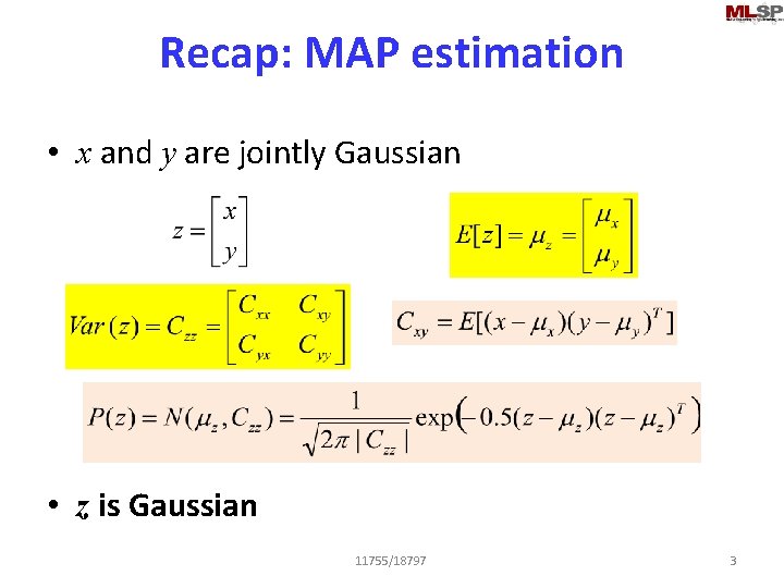
Recap: MAP estimation • x and y are jointly Gaussian • z is Gaussian 11755/18797 3

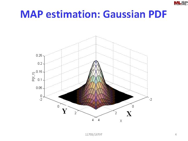
MAP estimation: Gaussian PDF F 1 Y X 11755/18797 4

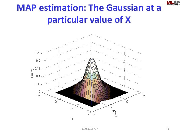
MAP estimation: The Gaussian at a particular value of X x 0 11755/18797 5

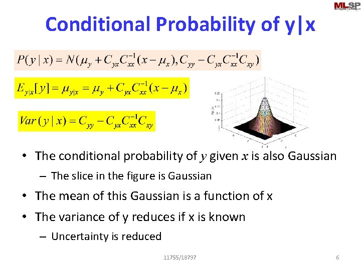
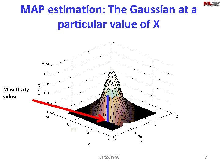
Conditional Probability of y|x • The conditional probability of y given x is also Gaussian – The slice in the figure is Gaussian • The mean of this Gaussian is a function of x • The variance of y reduces if x is known – Uncertainty is reduced 11755/18797 6

MAP estimation: The Gaussian at a particular value of X Most likely value F 1 x 0 11755/18797 7

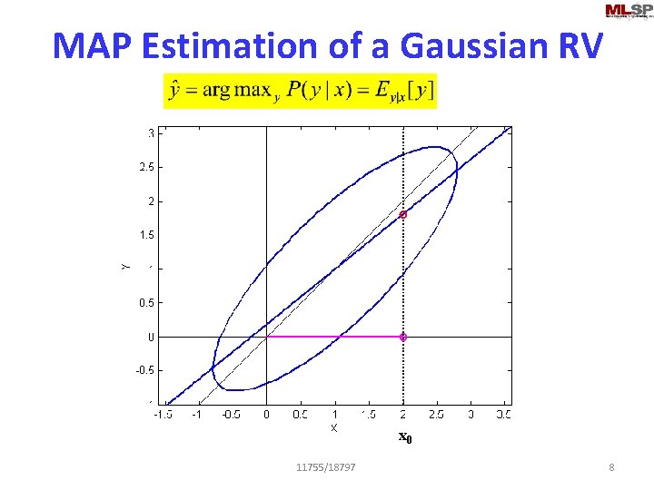
MAP Estimation of a Gaussian RV x 0 11755/18797 8

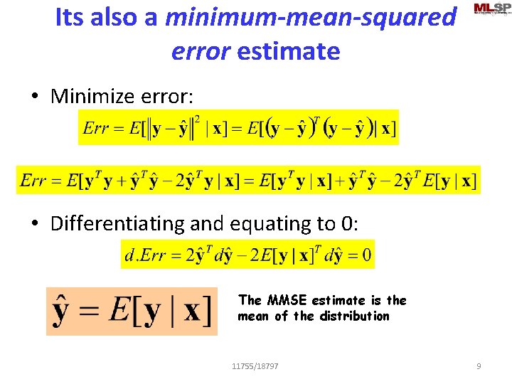
Its also a minimum-mean-squared error estimate • Minimize error: • Differentiating and equating to 0: The MMSE estimate is the mean of the distribution 11755/18797 9

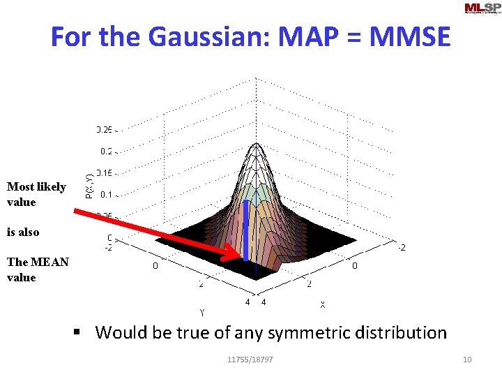
For the Gaussian: MAP = MMSE Most likely value is also The MEAN value § Would be true of any symmetric distribution 11755/18797 10

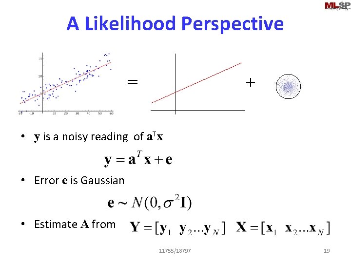
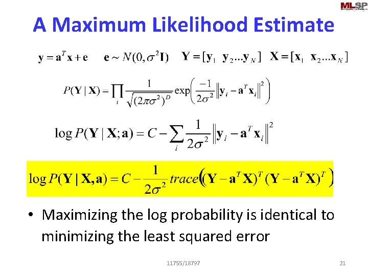
A Likelihood Perspective = + • y is a noisy reading of a. Tx • Error e is Gaussian • Estimate A from 11755/18797 19

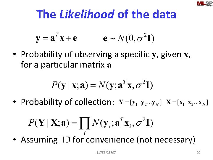
The Likelihood of the data • Probability of observing a specific y, given x, for a particular matrix a • Probability of collection: • Assuming IID for convenience (not necessary) 11755/18797 20

A Maximum Likelihood Estimate • Maximizing the log probability is identical to minimizing the least squared error 11755/18797 21

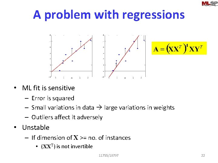
A problem with regressions • ML fit is sensitive – Error is squared – Small variations in data large variations in weights – Outliers affect it adversely • Unstable – If dimension of X >= no. of instances • (XXT) is not invertible 11755/18797 22

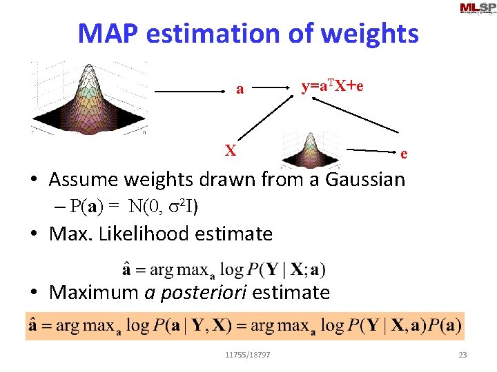
MAP estimation of weights a y=a. TX+e X e • Assume weights drawn from a Gaussian – P(a) = N(0, s 2 I) • Max. Likelihood estimate • Maximum a posteriori estimate 11755/18797 23

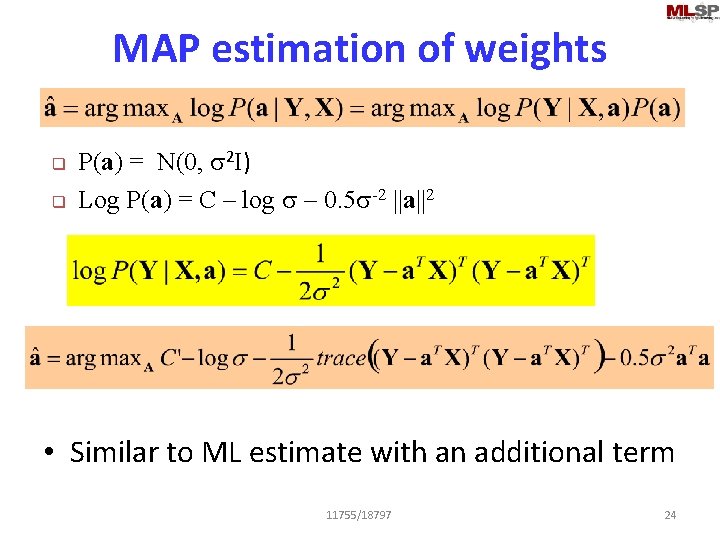
MAP estimation of weights q q P(a) = N(0, s 2 I) Log P(a) = C – log s – 0. 5 s-2 ||a||2 • Similar to ML estimate with an additional term 11755/18797 24

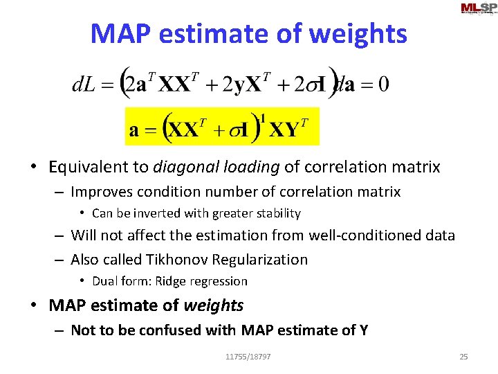
MAP estimate of weights • Equivalent to diagonal loading of correlation matrix – Improves condition number of correlation matrix • Can be inverted with greater stability – Will not affect the estimation from well-conditioned data – Also called Tikhonov Regularization • Dual form: Ridge regression • MAP estimate of weights – Not to be confused with MAP estimate of Y 11755/18797 25

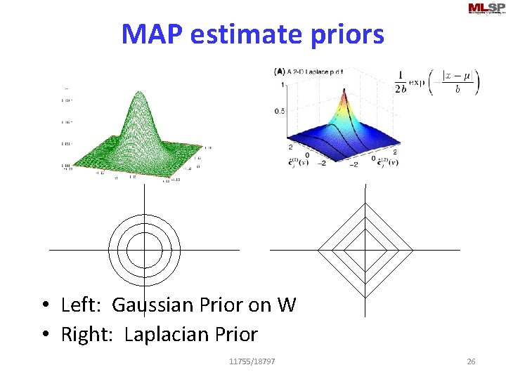
MAP estimate priors • Left: Gaussian Prior on W • Right: Laplacian Prior 11755/18797 26

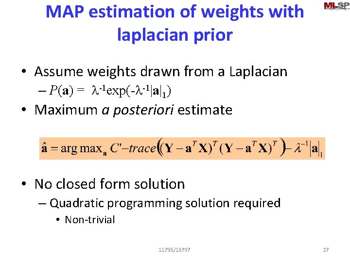
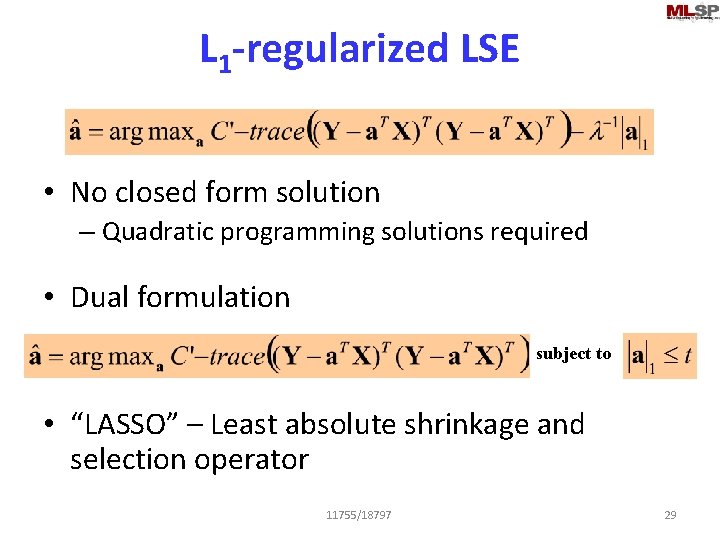
MAP estimation of weights with laplacian prior • Assume weights drawn from a Laplacian – P(a) = l-1 exp(-l-1|a|1) • Maximum a posteriori estimate • No closed form solution – Quadratic programming solution required • Non-trivial 11755/18797 27

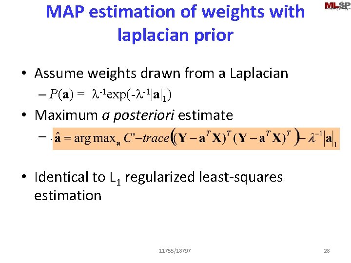
MAP estimation of weights with laplacian prior • Assume weights drawn from a Laplacian – P(a) = l-1 exp(-l-1|a|1) • Maximum a posteriori estimate –… • Identical to L 1 regularized least-squares estimation 11755/18797 28

L 1 -regularized LSE • No closed form solution – Quadratic programming solutions required • Dual formulation subject to • “LASSO” – Least absolute shrinkage and selection operator 11755/18797 29

LASSO Algorithms • Various convex optimization algorithms • LARS: Least angle regression • Pathwise coordinate descent. . • Matlab code available from web 11755/18797 30

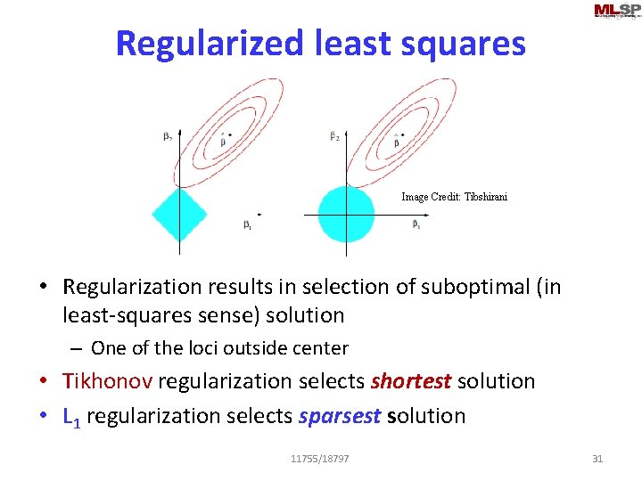
Regularized least squares Image Credit: Tibshirani • Regularization results in selection of suboptimal (in least-squares sense) solution – One of the loci outside center • Tikhonov regularization selects shortest solution • L 1 regularization selects sparsest solution 11755/18797 31

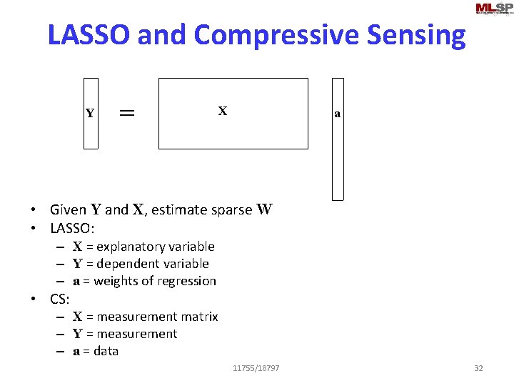
LASSO and Compressive Sensing Y = X a • Given Y and X, estimate sparse W • LASSO: – X = explanatory variable – Y = dependent variable – a = weights of regression • CS: – X = measurement matrix – Y = measurement – a = data 11755/18797 32

MAP / ML / MMSE • General statistical estimators • All used to predict a variable, based on other parameters related to it. . • Most common assumption: Data are Gaussian, all RVs are Gaussian – Other probability densities may also be used. . • For Gaussians relationships are linear as we saw. . 11755/18797 33

Gaussians and more Gaussians. . • Linear Gaussian Models. . • But first a recap 11755/18797 34

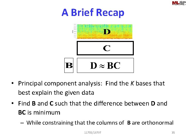
A Brief Recap • Principal component analysis: Find the K bases that best explain the given data • Find B and C such that the difference between D and BC is minimum – While constraining that the columns of B are orthonormal 11755/18797 35

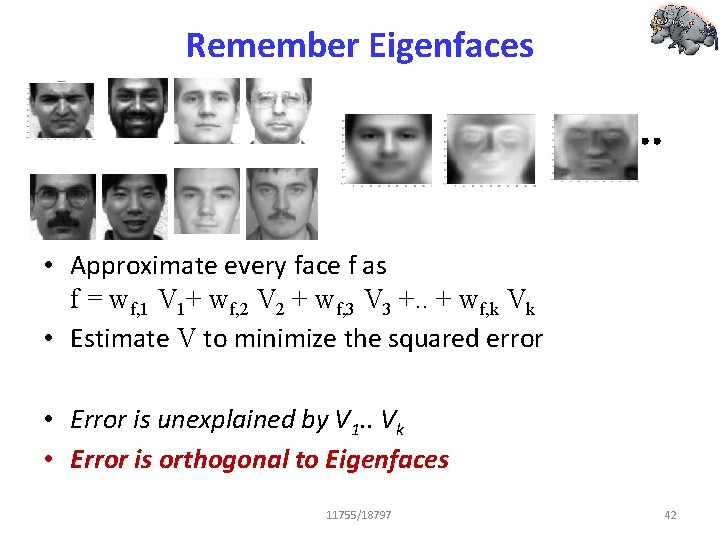
Remember Eigenfaces • Approximate every face f as f = wf, 1 V 1+ wf, 2 V 2 + wf, 3 V 3 +. . + wf, k Vk • Estimate V to minimize the squared error • Error is unexplained by V 1. . Vk • Error is orthogonal to Eigenfaces 11755/18797 36

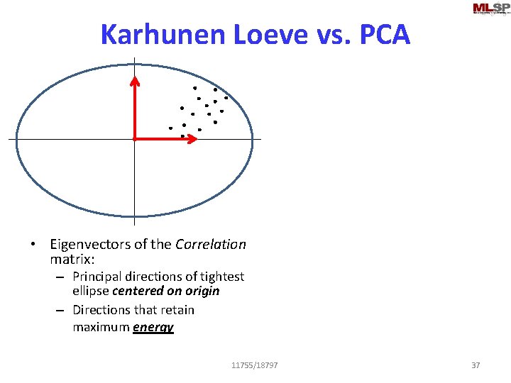
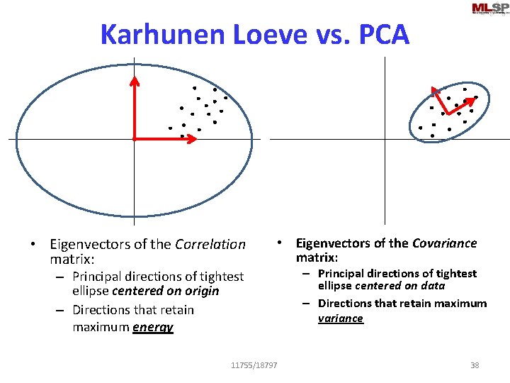
Karhunen Loeve vs. PCA • Eigenvectors of the Correlation matrix: – Principal directions of tightest ellipse centered on origin – Directions that retain maximum energy 11755/18797 37

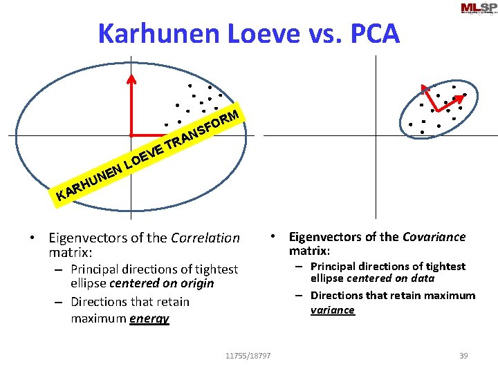
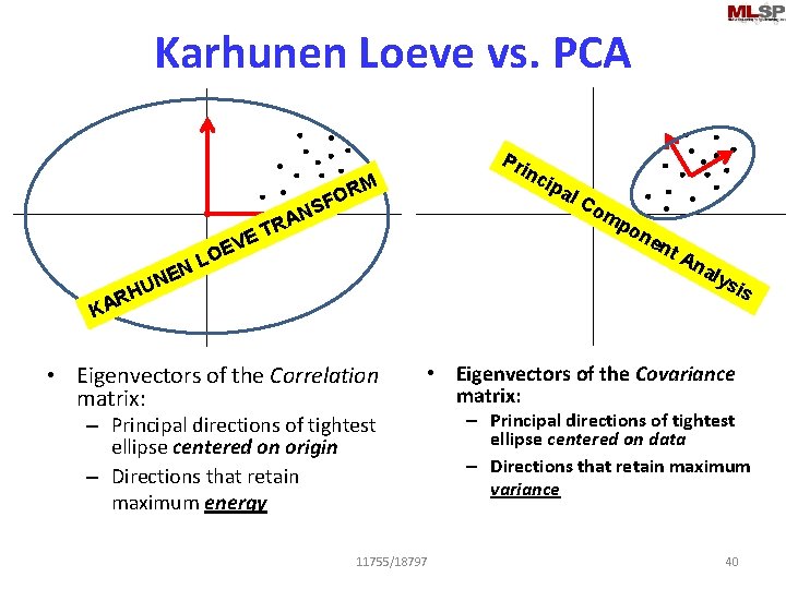
Karhunen Loeve vs. PCA • Eigenvectors of the Correlation matrix: • Eigenvectors of the Covariance matrix: – Principal directions of tightest ellipse centered on origin – Directions that retain maximum energy 11755/18797 – Principal directions of tightest ellipse centered on data – Directions that retain maximum variance 38

Karhunen Loeve vs. PCA M RA T E OR F S N V N NE U RH E LO KA • Eigenvectors of the Correlation matrix: • Eigenvectors of the Covariance matrix: – Principal directions of tightest ellipse centered on origin – Directions that retain maximum energy 11755/18797 – Principal directions of tightest ellipse centered on data – Directions that retain maximum variance 39

Karhunen Loeve vs. PCA O SF Pr inc RM om AN R ET V OE L EN UN H R KA • Eigenvectors of the Correlation matrix: ipa l. C po ne nt An aly sis • Eigenvectors of the Covariance matrix: – Principal directions of tightest ellipse centered on origin – Directions that retain maximum energy 11755/18797 – Principal directions of tightest ellipse centered on data – Directions that retain maximum variance 40

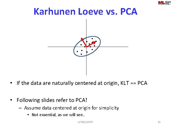
Karhunen Loeve vs. PCA • If the data are naturally centered at origin, KLT == PCA • Following slides refer to PCA! – Assume data centered at origin for simplicity • Not essential, as we will see. . 11755/18797 41

Remember Eigenfaces • Approximate every face f as f = wf, 1 V 1+ wf, 2 V 2 + wf, 3 V 3 +. . + wf, k Vk • Estimate V to minimize the squared error • Error is unexplained by V 1. . Vk • Error is orthogonal to Eigenfaces 11755/18797 42

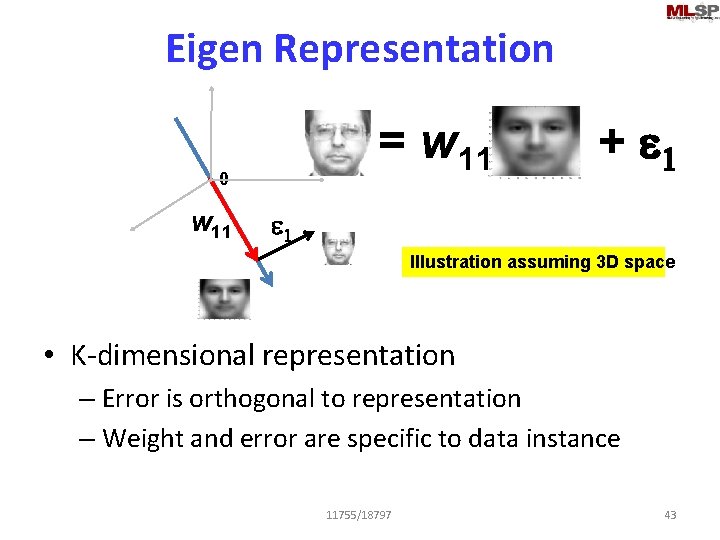
Eigen Representation = w 11 0 w 11 + e 1 Illustration assuming 3 D space • K-dimensional representation – Error is orthogonal to representation – Weight and error are specific to data instance 11755/18797 43

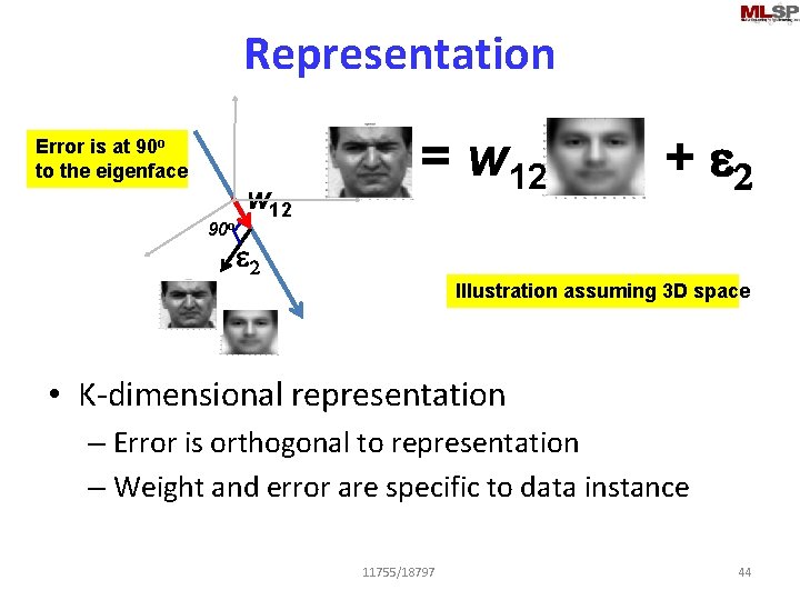
Representation Error is at 90 o to the eigenface 90 o w 12 = w 12 + e 2 Illustration assuming 3 D space • K-dimensional representation – Error is orthogonal to representation – Weight and error are specific to data instance 11755/18797 44

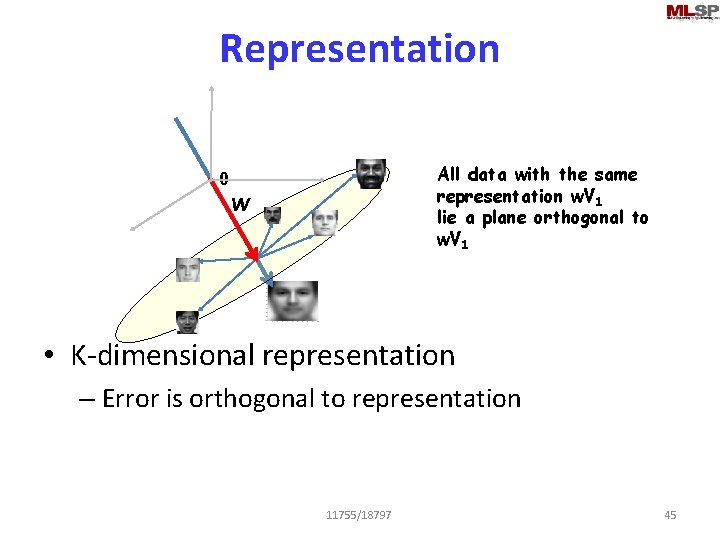
Representation All data with the same representation w. V 1 lie a plane orthogonal to w. V 1 0 w • K-dimensional representation – Error is orthogonal to representation 11755/18797 45

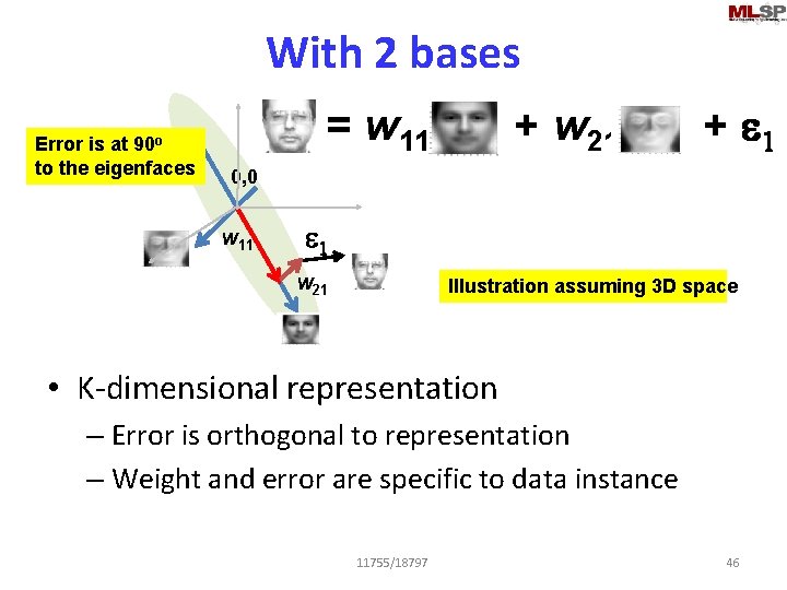
With 2 bases Error is at 90 o to the eigenfaces = w 11 + w 21 + e 1 0, 0 w 11 e 1 w 21 Illustration assuming 3 D space • K-dimensional representation – Error is orthogonal to representation – Weight and error are specific to data instance 11755/18797 46

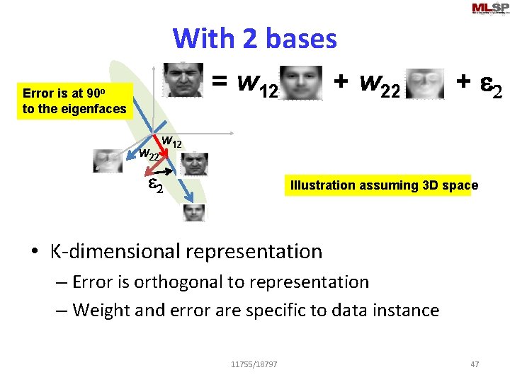
With 2 bases = w 12 Error is at 90 o to the eigenfaces w 22 + e 2 w 12 e 2 Illustration assuming 3 D space • K-dimensional representation – Error is orthogonal to representation – Weight and error are specific to data instance 11755/18797 47

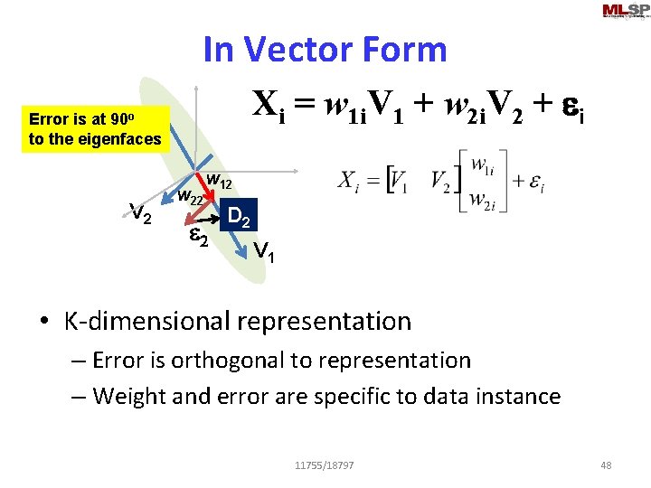
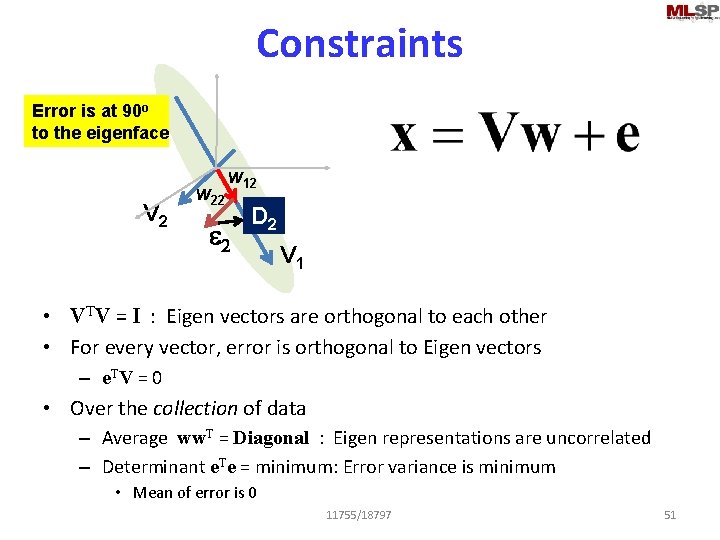
In Vector Form Xi = w 1 i. V 1 + w 2 i. V 2 + ei Error is at 90 o to the eigenfaces V 2 w 22 w 12 e 2 D 2 V 1 • K-dimensional representation – Error is orthogonal to representation – Weight and error are specific to data instance 11755/18797 48

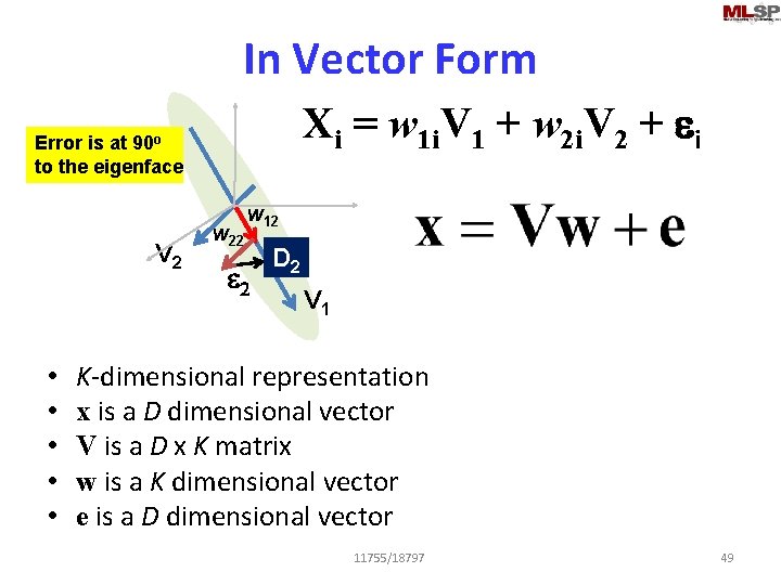
In Vector Form Xi = w 1 i. V 1 + w 2 i. V 2 + ei Error is at 90 o to the eigenface V 2 • • • w 22 w 12 e 2 D 2 V 1 K-dimensional representation x is a D dimensional vector V is a D x K matrix w is a K dimensional vector e is a D dimensional vector 11755/18797 49

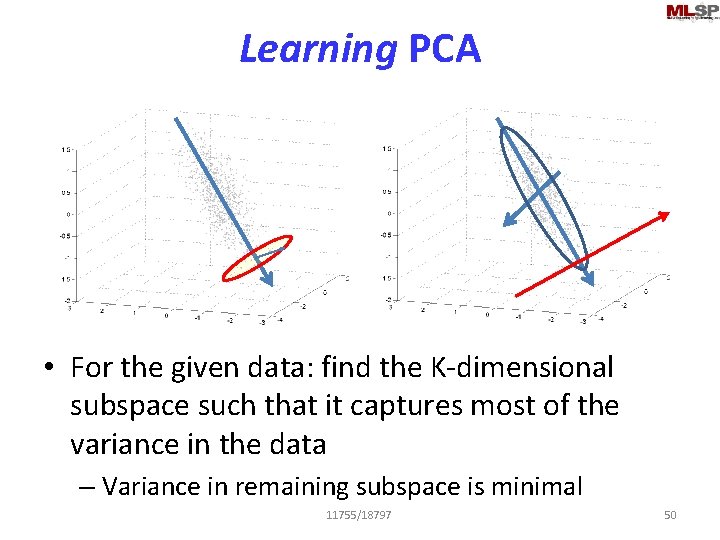
Learning PCA • For the given data: find the K-dimensional subspace such that it captures most of the variance in the data – Variance in remaining subspace is minimal 11755/18797 50

Constraints Error is at 90 o to the eigenface V 2 w 22 w 12 e 2 D 2 V 1 • VTV = I : Eigen vectors are orthogonal to each other • For every vector, error is orthogonal to Eigen vectors – e. T V = 0 • Over the collection of data – Average ww. T = Diagonal : Eigen representations are uncorrelated – Determinant e. Te = minimum: Error variance is minimum • Mean of error is 0 11755/18797 51

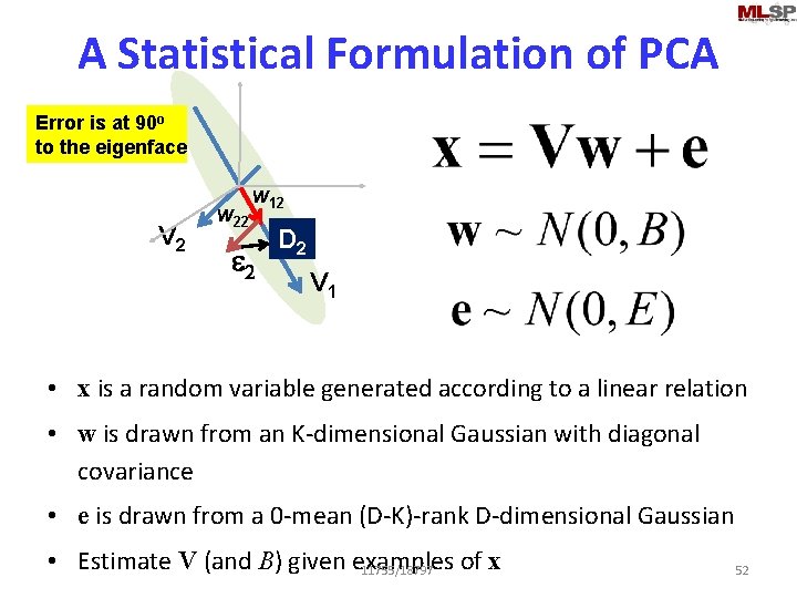
A Statistical Formulation of PCA Error is at 90 o to the eigenface V 2 w 22 w 12 e 2 D 2 V 1 • x is a random variable generated according to a linear relation • w is drawn from an K-dimensional Gaussian with diagonal covariance • e is drawn from a 0 -mean (D-K)-rank D-dimensional Gaussian • Estimate V (and B) given examples of x 11755/18797 52

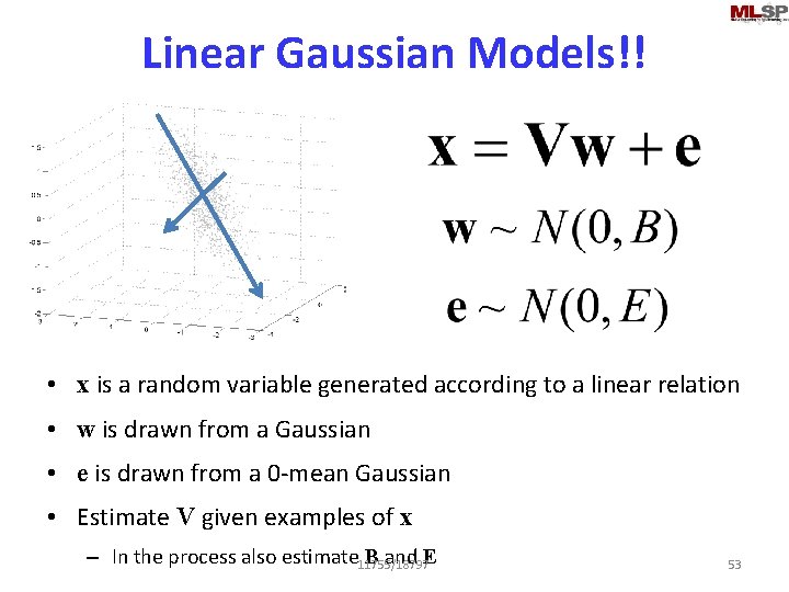
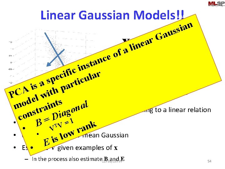
Linear Gaussian Models!! • x is a random variable generated according to a linear relation • w is drawn from a Gaussian • e is drawn from a 0 -mean Gaussian • Estimate V given examples of x – In the process also estimate 11755/18797 B and E 53

Linear Gaussian Models!! a G ar n a i uss e n i l a f o e c n a t s n i c i f r i c a l e u p c s i t a r s a i p A h t C i P w l e d s t o l n i a m a n • x is satrandom variable generated according to a linear relation r o g on = Dia I c • w is drawn = a Gaussian B VTfrom k V n a • • r w • e is drawn from a 0 -mean Gaussian o l s i EV given examples of x • Estimate • – In the process also estimate 11755/18797 B and E 54

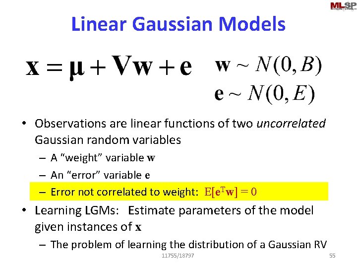
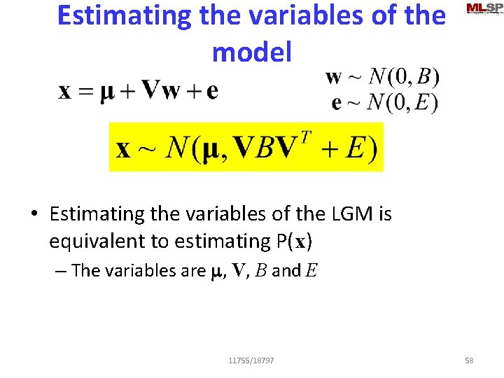
Linear Gaussian Models • Observations are linear functions of two uncorrelated Gaussian random variables – A “weight” variable w – An “error” variable e – Error not correlated to weight: E[e. Tw] = 0 • Learning LGMs: Estimate parameters of the model given instances of x – The problem of learning the distribution of a Gaussian RV 11755/18797 55

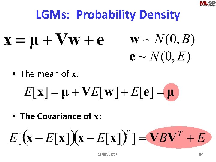
LGMs: Probability Density • The mean of x: • The Covariance of x: 11755/18797 56

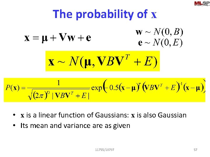
The probability of x • x is a linear function of Gaussians: x is also Gaussian • Its mean and variance are as given 11755/18797 57

Estimating the variables of the model • Estimating the variables of the LGM is equivalent to estimating P(x) – The variables are m, V, B and E 11755/18797 58

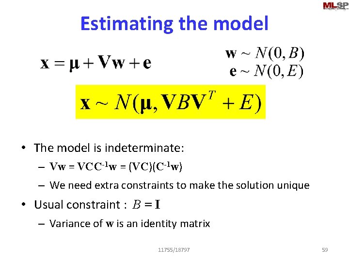
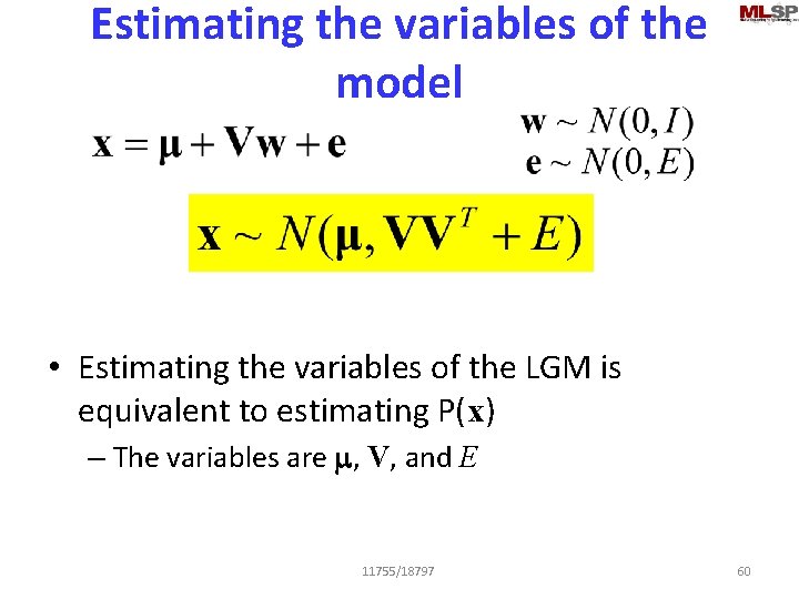
Estimating the model • The model is indeterminate: – Vw = VCC-1 w = (VC)(C-1 w) – We need extra constraints to make the solution unique • Usual constraint : B = I – Variance of w is an identity matrix 11755/18797 59

Estimating the variables of the model • Estimating the variables of the LGM is equivalent to estimating P(x) – The variables are m, V, and E 11755/18797 60

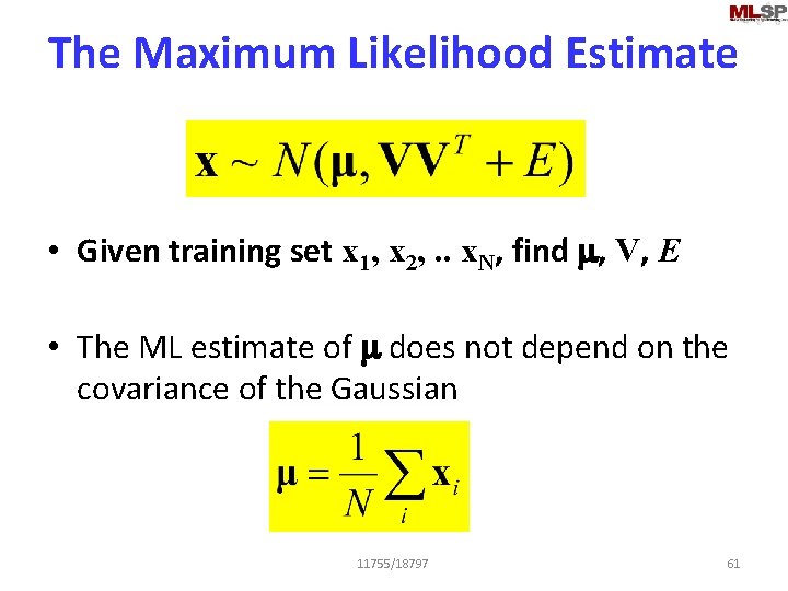
The Maximum Likelihood Estimate • Given training set x 1, x 2, . . x. N, find m, V, E • The ML estimate of m does not depend on the covariance of the Gaussian 11755/18797 61

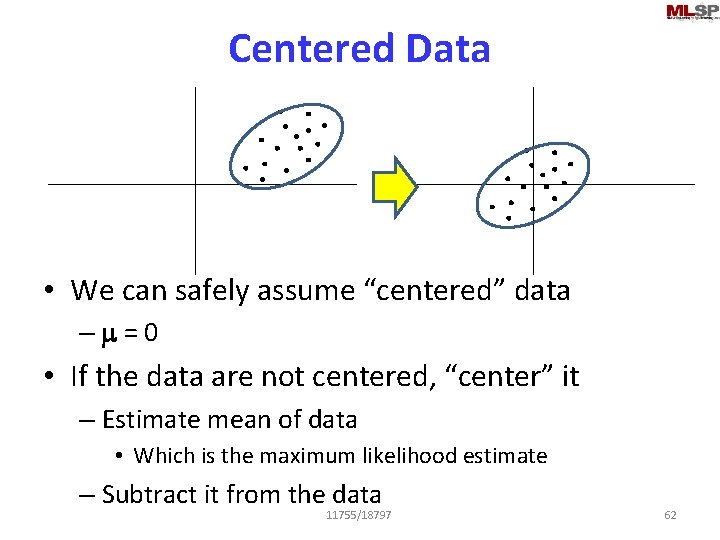
Centered Data • We can safely assume “centered” data –m=0 • If the data are not centered, “center” it – Estimate mean of data • Which is the maximum likelihood estimate – Subtract it from the data 11755/18797 62

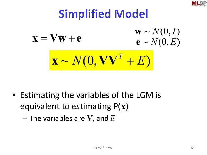
Simplified Model • Estimating the variables of the LGM is equivalent to estimating P(x) – The variables are V, and E 11755/18797 63

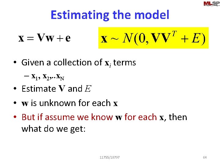
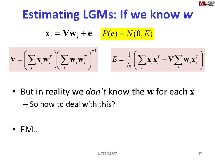
Estimating the model • Given a collection of xi terms – x 1, x 2, . . x. N • Estimate V and E • w is unknown for each x • But if assume we know w for each x, then what do we get: 11755/18797 64

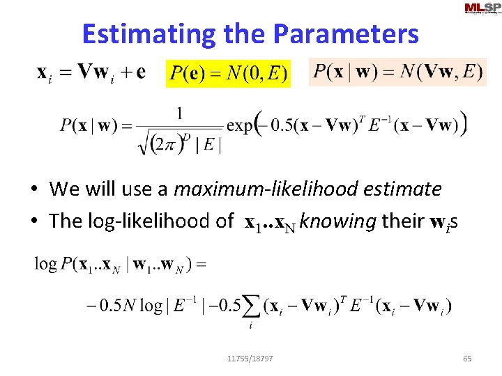
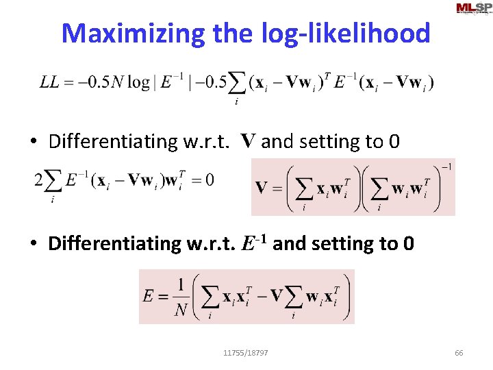
Estimating the Parameters • We will use a maximum-likelihood estimate • The log-likelihood of x 1. . x. N knowing their wis 11755/18797 65

Maximizing the log-likelihood • Differentiating w. r. t. V and setting to 0 • Differentiating w. r. t. E-1 and setting to 0 11755/18797 66

Estimating LGMs: If we know w • But in reality we don’t know the w for each x – So how to deal with this? • EM. . 11755/18797 67

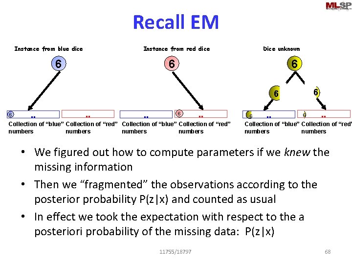
Recall EM Instance from blue dice Instance from red dice 6 Dice unknown 6 6 6 . . Collection of “blue” Collection of “red” numbers 6 . . Collection of “blue” Collection of “red” numbers • We figured out how to compute parameters if we knew the missing information • Then we “fragmented” the observations according to the posterior probability P(z|x) and counted as usual • In effect we took the expectation with respect to the a posteriori probability of the missing data: P(z|x) 11755/18797 68

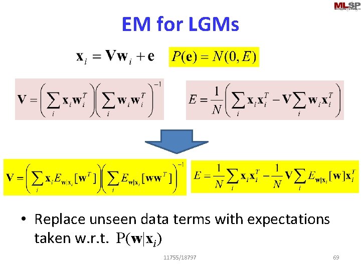
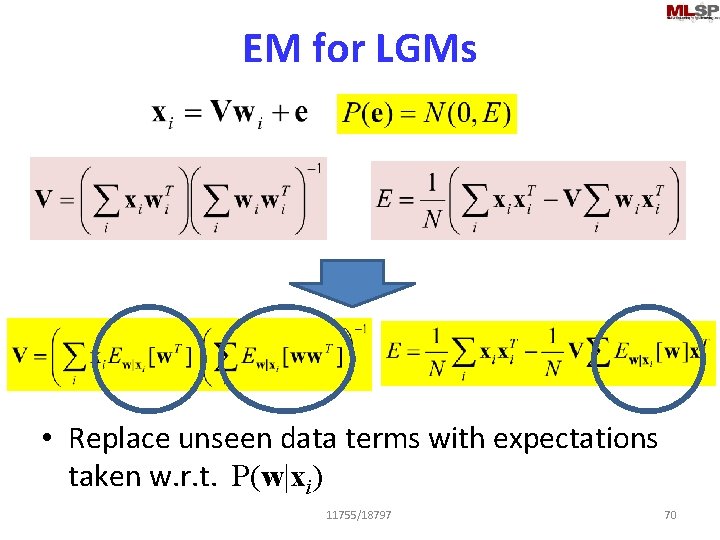
EM for LGMs • Replace unseen data terms with expectations taken w. r. t. P(w|xi) 11755/18797 69

EM for LGMs • Replace unseen data terms with expectations taken w. r. t. P(w|xi) 11755/18797 70

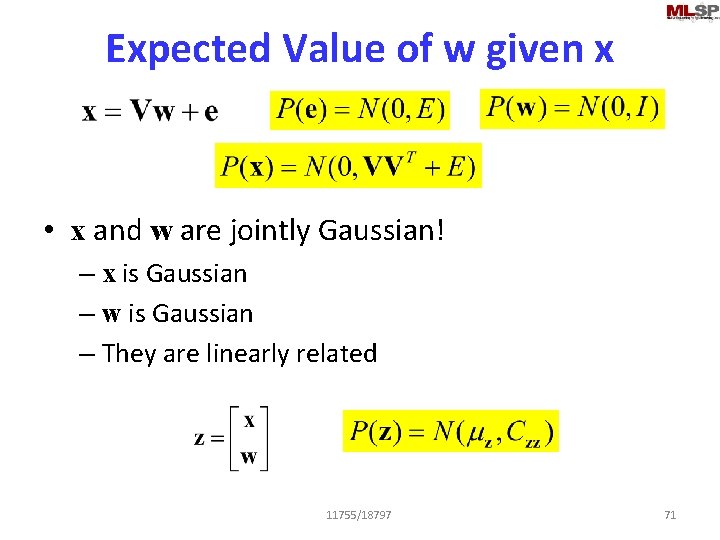
Expected Value of w given x • x and w are jointly Gaussian! – x is Gaussian – w is Gaussian – They are linearly related 11755/18797 71

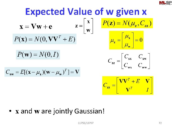
Expected Value of w given x • x and w are jointly Gaussian! 11755/18797 72

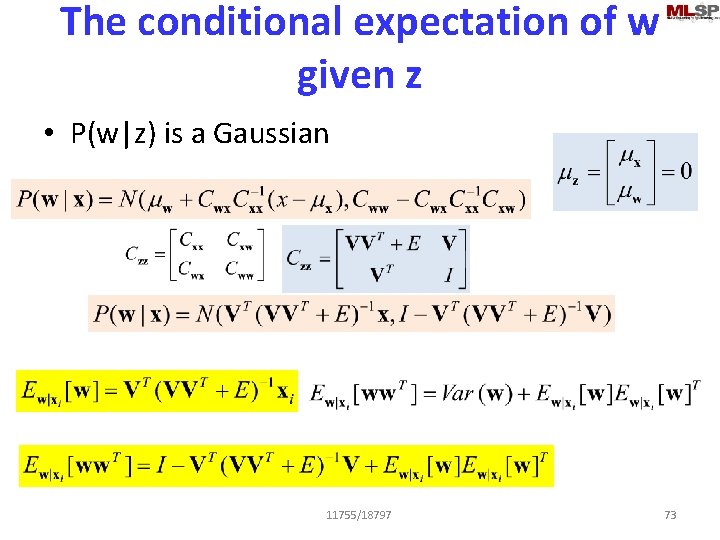
The conditional expectation of w given z • P(w|z) is a Gaussian 11755/18797 73

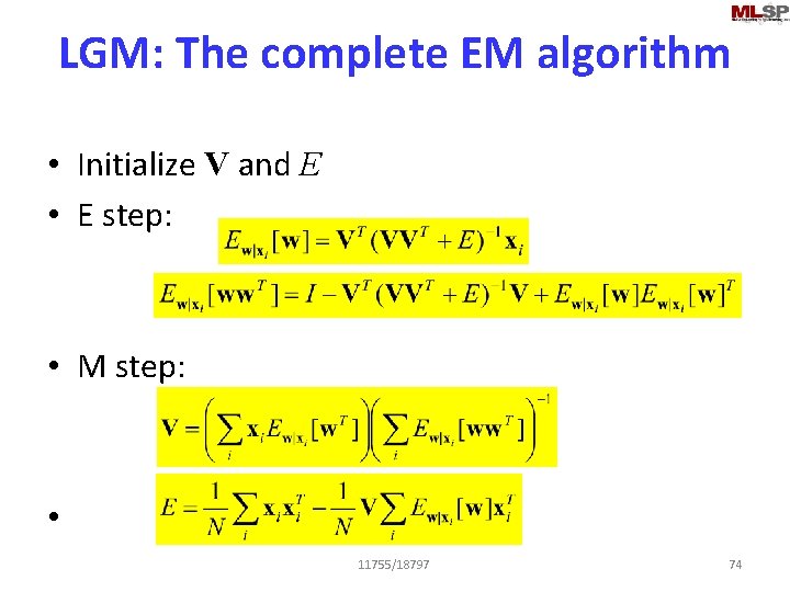
LGM: The complete EM algorithm • Initialize V and E • E step: • M step: • 11755/18797 74

So what have we achieved • Employed a complicated EM algorithm to learn a Gaussian PDF for a variable x • What have we gained? ? ? • Next class: – PCA • Sensible PCA • EM algorithms for PCA – Factor Analysis • FA for feature extraction 11755/18797 75

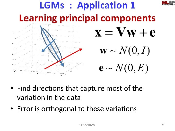
LGMs : Application 1 Learning principal components • Find directions that capture most of the variation in the data • Error is orthogonal to these variations 11755/18797 76

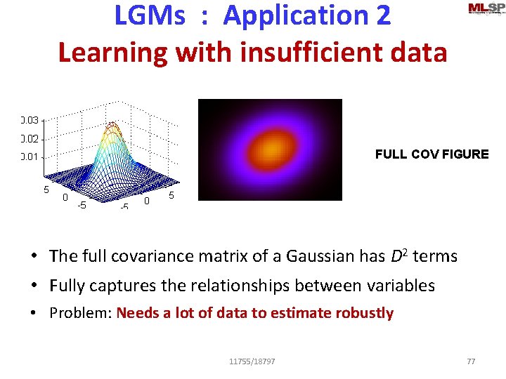
LGMs : Application 2 Learning with insufficient data FULL COV FIGURE • The full covariance matrix of a Gaussian has D 2 terms • Fully captures the relationships between variables • Problem: Needs a lot of data to estimate robustly 11755/18797 77

To be continued. . • Other applications. . • Next class 11755/18797 78