Machine Learning for Signal Processing Fundamentals of Linear

Machine Learning for Signal Processing Fundamentals of Linear Algebra - 2 Class 3. 5 Sep 2013 Instructor: Bhiksha Raj 5 Sep 2013 11 -755/18 -797 1

Overview • • Vectors and matrices Basic vector/matrix operations Various matrix types Projections • • • More on matrix types Matrix determinants Matrix inversion Eigenanalysis Singular value decomposition 5 Sep 2013 11 -755/18 -797 2

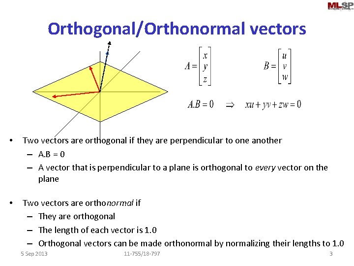
Orthogonal/Orthonormal vectors • Two vectors are orthogonal if they are perpendicular to one another – A. B = 0 – A vector that is perpendicular to a plane is orthogonal to every vector on the plane • Two vectors are orthonormal if – They are orthogonal – The length of each vector is 1. 0 – Orthogonal vectors can be made orthonormal by normalizing their lengths to 1. 0 5 Sep 2013 11 -755/18 -797 3

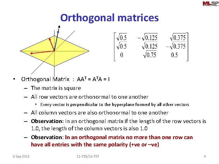
Orthogonal matrices • Orthogonal Matrix : AAT = ATA = I – The matrix is square – All row vectors are orthonormal to one another • Every vector is perpendicular to the hyperplane formed by all other vectors – All column vectors are also orthonormal to one another – Observation: In an orthogonal matrix if the length of the row vectors is 1. 0, the length of the column vectors is also 1. 0 – Observation: In an orthogonal matrix no more than one row can have all entries with the same polarity (+ve or –ve) 5 Sep 2013 11 -755/18 -797 4

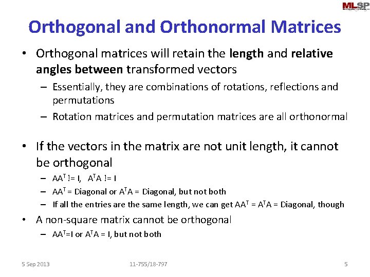
Orthogonal and Orthonormal Matrices • Orthogonal matrices will retain the length and relative angles between transformed vectors – Essentially, they are combinations of rotations, reflections and permutations – Rotation matrices and permutation matrices are all orthonormal • If the vectors in the matrix are not unit length, it cannot be orthogonal – AAT != I, ATA != I – AAT = Diagonal or ATA = Diagonal, but not both – If all the entries are the same length, we can get AAT = ATA = Diagonal, though • A non-square matrix cannot be orthogonal – AAT=I or ATA = I, but not both 5 Sep 2013 11 -755/18 -797 5

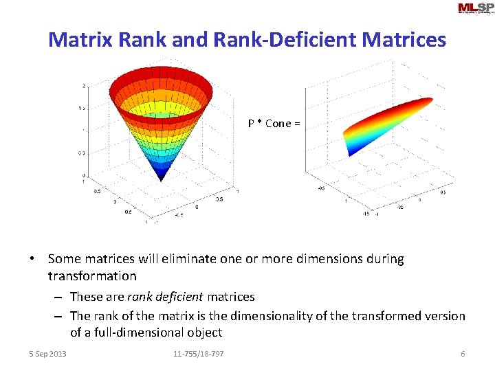
Matrix Rank and Rank-Deficient Matrices P * Cone = • Some matrices will eliminate one or more dimensions during transformation – These are rank deficient matrices – The rank of the matrix is the dimensionality of the transformed version of a full-dimensional object 5 Sep 2013 11 -755/18 -797 6

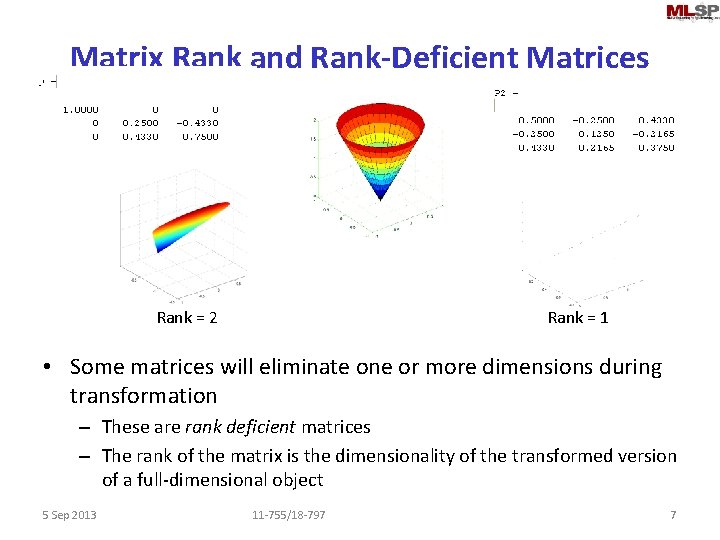
Matrix Rank and Rank-Deficient Matrices Rank = 2 Rank = 1 • Some matrices will eliminate one or more dimensions during transformation – These are rank deficient matrices – The rank of the matrix is the dimensionality of the transformed version of a full-dimensional object 5 Sep 2013 11 -755/18 -797 7

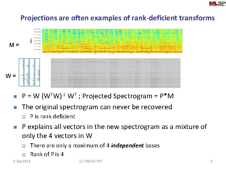
Projections are often examples of rank-deficient transforms M = W = n n P = W (WTW)-1 WT ; Projected Spectrogram = P*M The original spectrogram can never be recovered q n P is rank deficient P explains all vectors in the new spectrogram as a mixture of only the 4 vectors in W q q There are only a maximum of 4 independent bases Rank of P is 4 5 Sep 2013 11 -755/18 -797 8

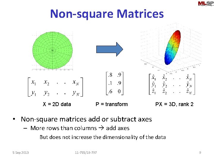
Non-square Matrices X = 2 D data P = transform PX = 3 D, rank 2 • Non-square matrices add or subtract axes – More rows than columns add axes • But does not increase the dimensionality of the dataaxes • May reduce dimensionality of the data 5 Sep 2013 11 -755/18 -797 9

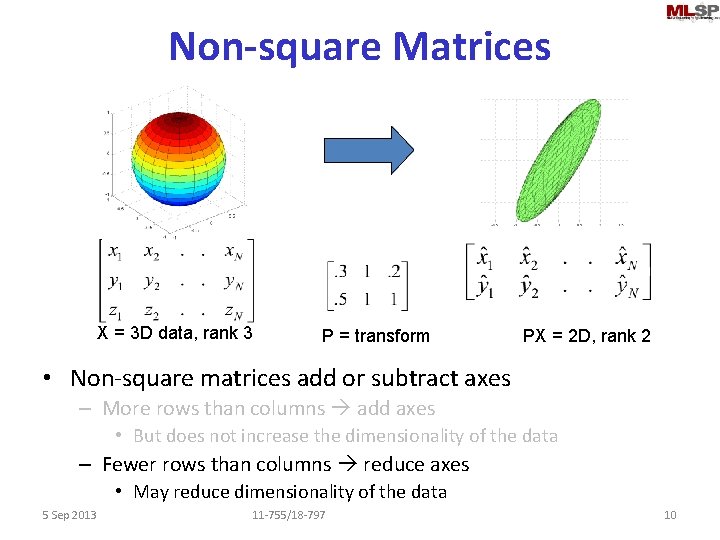
Non-square Matrices X = 3 D data, rank 3 P = transform PX = 2 D, rank 2 • Non-square matrices add or subtract axes – More rows than columns add axes • But does not increase the dimensionality of the data – Fewer rows than columns reduce axes • May reduce dimensionality of the data 5 Sep 2013 11 -755/18 -797 10

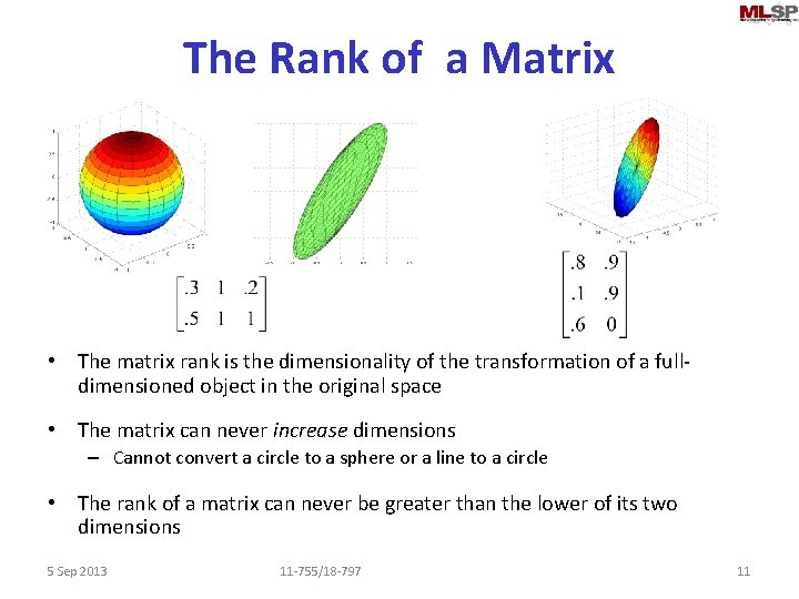
The Rank of a Matrix • The matrix rank is the dimensionality of the transformation of a fulldimensioned object in the original space • The matrix can never increase dimensions – Cannot convert a circle to a sphere or a line to a circle • The rank of a matrix can never be greater than the lower of its two dimensions 5 Sep 2013 11 -755/18 -797 11

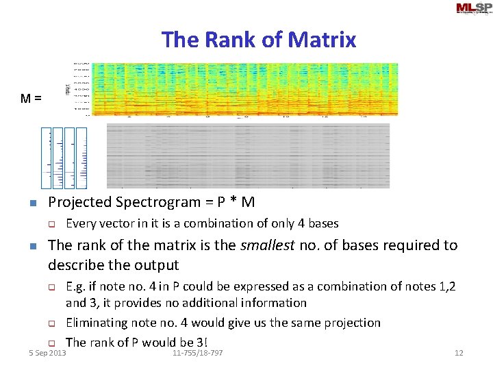
The Rank of Matrix M = n Projected Spectrogram = P * M q n Every vector in it is a combination of only 4 bases The rank of the matrix is the smallest no. of bases required to describe the output q q E. g. if note no. 4 in P could be expressed as a combination of notes 1, 2 and 3, it provides no additional information Eliminating note no. 4 would give us the same projection The rank of P would be 3! q 5 Sep 2013 11 -755/18 -797 12

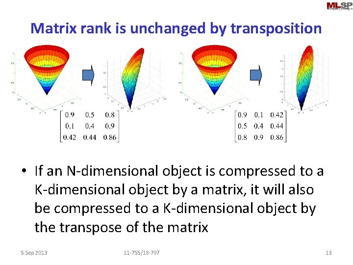
Matrix rank is unchanged by transposition • If an N-dimensional object is compressed to a K-dimensional object by a matrix, it will also be compressed to a K-dimensional object by the transpose of the matrix 5 Sep 2013 11 -755/18 -797 13

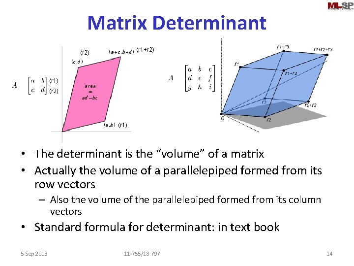
Matrix Determinant (r 1+r 2) (r 1) (r 2) (r 1) • The determinant is the “volume” of a matrix • Actually the volume of a parallelepiped formed from its row vectors – Also the volume of the parallelepiped formed from its column vectors • Standard formula for determinant: in text book 5 Sep 2013 11 -755/18 -797 14

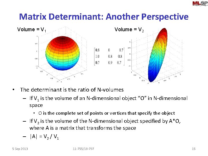
Matrix Determinant: Another Perspective Volume = V 1 Volume = V 2 • The determinant is the ratio of N-volumes – If V 1 is the volume of an N-dimensional object “O” in N-dimensional space • O is the complete set of points or vertices that specify the object – If V 2 is the volume of the N-dimensional object specified by A*O, where A is a matrix that transforms the space – |A| = V 2 / V 1 5 Sep 2013 11 -755/18 -797 15

Matrix Determinants • Matrix determinants are only defined for square matrices – They characterize volumes in linearly transformed space of the same dimensionality as the vectors • Rank deficient matrices have determinant 0 – Since they compress full-volumed N-dimensional objects into zerovolume N-dimensional objects • E. g. a 3 -D sphere into a 2 -D ellipse: The ellipse has 0 volume (although it does have area) • Conversely, all matrices of determinant 0 are rank deficient – Since they compress full-volumed N-dimensional objects into zero-volume objects 5 Sep 2013 11 -755/18 -797 16

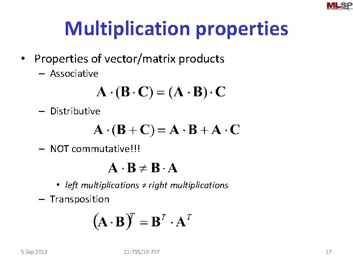
Multiplication properties • Properties of vector/matrix products – Associative – Distributive – NOT commutative!!! • left multiplications ≠ right multiplications – Transposition 5 Sep 2013 11 -755/18 -797 17

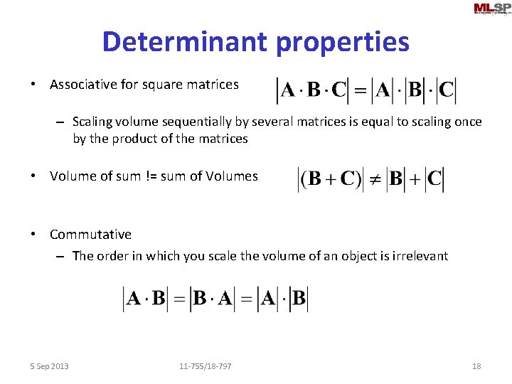
Determinant properties • Associative for square matrices – Scaling volume sequentially by several matrices is equal to scaling once by the product of the matrices • Volume of sum != sum of Volumes • Commutative – The order in which you scale the volume of an object is irrelevant 5 Sep 2013 11 -755/18 -797 18

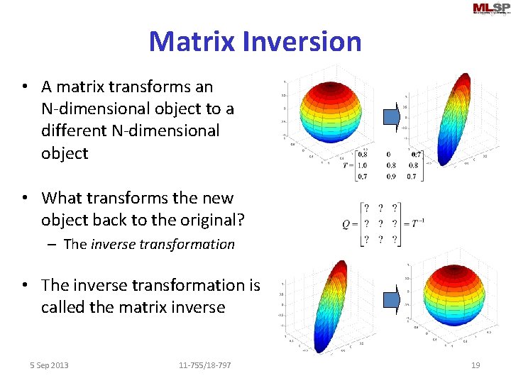
Matrix Inversion • A matrix transforms an N-dimensional object to a different N-dimensional object • What transforms the new object back to the original? – The inverse transformation • The inverse transformation is called the matrix inverse 5 Sep 2013 11 -755/18 -797 19

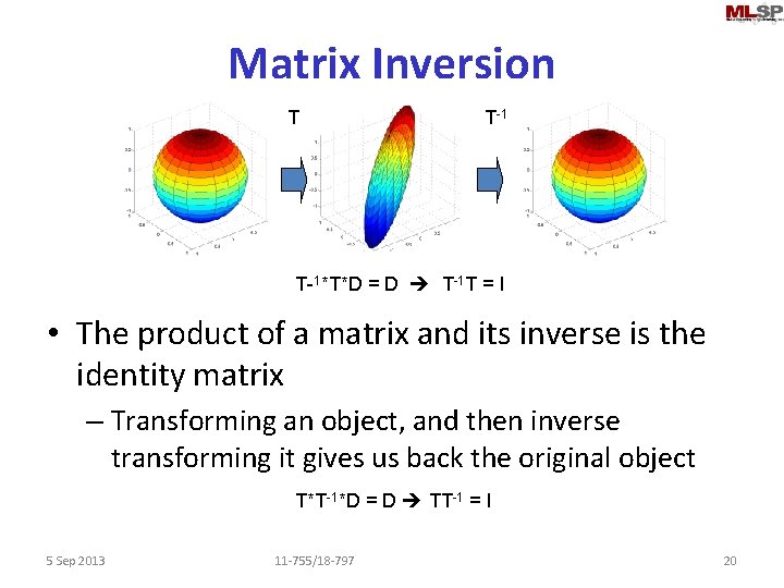
Matrix Inversion T T-1*T*D = D T-1 T = I • The product of a matrix and its inverse is the identity matrix – Transforming an object, and then inverse transforming it gives us back the original object T*T-1*D = D TT-1 = I 5 Sep 2013 11 -755/18 -797 20

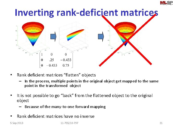
Inverting rank-deficient matrices • Rank deficient matrices “flatten” objects – In the process, multiple points in the original object get mapped to the same point in the transformed object • It is not possible to go “back” from the flattened object to the original object – Because of the many-to-one forward mapping • Rank deficient matrices have no inverse 5 Sep 2013 11 -755/18 -797 21

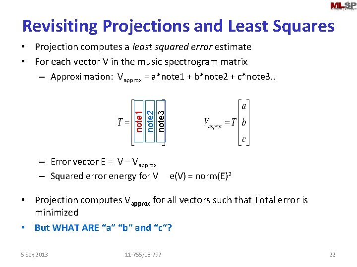
Revisiting Projections and Least Squares note 1 note 2 note 3 • Projection computes a least squared error estimate • For each vector V in the music spectrogram matrix – Approximation: Vapprox = a*note 1 + b*note 2 + c*note 3. . – Error vector E = V – Vapprox – Squared error energy for V e(V) = norm(E)2 • Projection computes Vapprox for all vectors such that Total error is minimized • But WHAT ARE “a” “b” and “c”? 5 Sep 2013 11 -755/18 -797 22

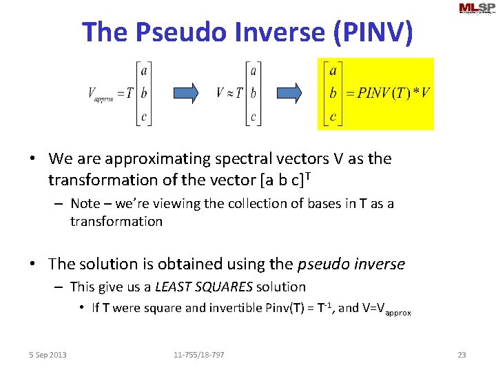
The Pseudo Inverse (PINV) • We are approximating spectral vectors V as the transformation of the vector [a b c]T – Note – we’re viewing the collection of bases in T as a transformation • The solution is obtained using the pseudo inverse – This give us a LEAST SQUARES solution • If T were square and invertible Pinv(T) = T-1, and V=Vapprox 5 Sep 2013 11 -755/18 -797 23

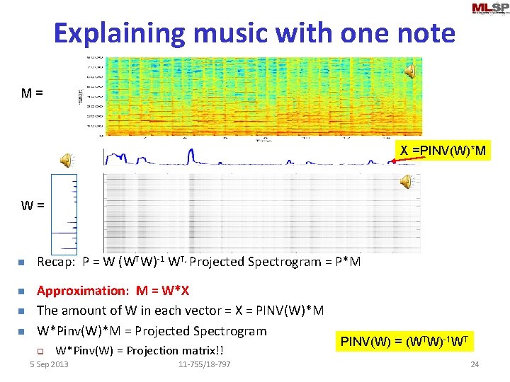
Explaining music with one note M = X =PINV(W)*M W = n n Recap: P = W (WTW)-1 WT, Projected Spectrogram = P*M Approximation: M = W*X The amount of W in each vector = X = PINV(W)*M W*Pinv(W)*M = Projected Spectrogram q W*Pinv(W) = Projection matrix!! 5 Sep 2013 11 -755/18 -797 PINV(W) = (WTW)-1 WT 24

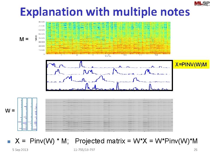
Explanation with multiple notes M = X=PINV(W)M W = n X = Pinv(W) * M; Projected matrix = W*X = W*Pinv(W)*M 5 Sep 2013 11 -755/18 -797 25

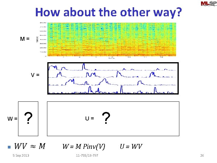
How about the other way? M = V = W = n ? U = ? W = M Pinv(V) U = WV 5 Sep 2013 11 -755/18 -797 26

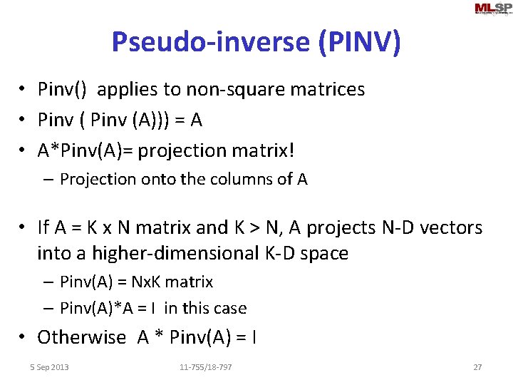
Pseudo-inverse (PINV) • Pinv() applies to non-square matrices • Pinv (A))) = A • A*Pinv(A)= projection matrix! – Projection onto the columns of A • If A = K x N matrix and K > N, A projects N-D vectors into a higher-dimensional K-D space – Pinv(A) = Nx. K matrix – Pinv(A)*A = I in this case • Otherwise A * Pinv(A) = I 5 Sep 2013 11 -755/18 -797 27

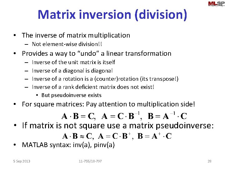
Matrix inversion (division) • The inverse of matrix multiplication – Not element-wise division!! • Provides a way to “undo” a linear transformation – – Inverse of the unit matrix is itself Inverse of a diagonal is diagonal Inverse of a rotation is a (counter)rotation (its transpose!) Inverse of a rank deficient matrix does not exist! • But pseudoinverse exists • For square matrices: Pay attention to multiplication side! • If matrix is not square use a matrix pseudoinverse: • MATLAB syntax: inv(a), pinv(a) 5 Sep 2013 11 -755/18 -797 28

Eigenanalysis • If something can go through a process mostly unscathed in character it is an eigen-something – Sound example: • A vector that can undergo a matrix multiplication and keep pointing the same way is an eigenvector – Its length can change though • How much its length changes is expressed by its corresponding eigenvalue – Each eigenvector of a matrix has its eigenvalue • Finding these “eigenthings” is called eigenanalysis 5 Sep 2013 11 -755/18 -797 29

Eigen. Vectors and Eigen. Values Black vectors are eigen vectors • Vectors that do not change angle upon transformation – They may change length – V = eigen vector – l = eigen value 5 Sep 2013 30

Eigen vector example 5 Sep 2013 11 -755/18 -797 31

Matrix multiplication revisited • Matrix transformation “transforms” the space – Warps the paper so that the normals to the two vectors now lie along the axes 5 Sep 2013 11 -755/18 -797 32

A stretching operation 1. 4 0. 8 • Draw two lines • Stretch / shrink the paper along these lines by factors l 1 and l 2 – The factors could be negative – implies flipping the paper • The result is a transformation of the space 5 Sep 2013 11 -755/18 -797 33

A stretching operation n n Draw two lines Stretch / shrink the paper along these lines by factors l 1 and l 2 q n The factors could be negative – implies flipping the paper The result is a transformation of the space 5 Sep 2013 11 -755/18 -797 34

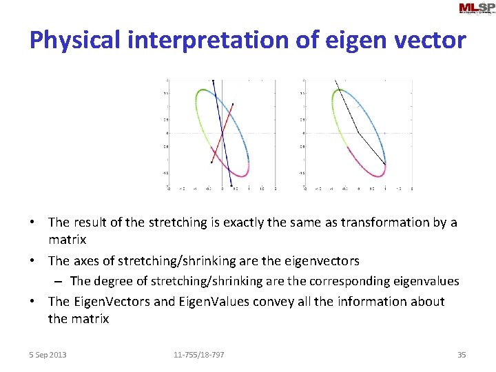
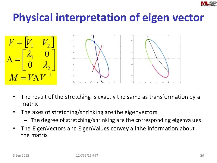
Physical interpretation of eigen vector • The result of the stretching is exactly the same as transformation by a matrix • The axes of stretching/shrinking are the eigenvectors – The degree of stretching/shrinking are the corresponding eigenvalues • The Eigen. Vectors and Eigen. Values convey all the information about the matrix 5 Sep 2013 11 -755/18 -797 35

Physical interpretation of eigen vector • The result of the stretching is exactly the same as transformation by a matrix • The axes of stretching/shrinking are the eigenvectors – The degree of stretching/shrinking are the corresponding eigenvalues • The Eigen. Vectors and Eigen. Values convey all the information about the matrix 5 Sep 2013 11 -755/18 -797 36

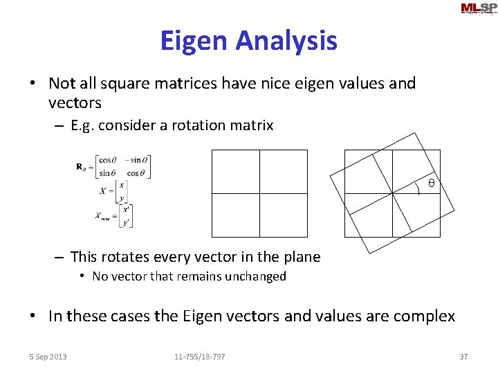
Eigen Analysis • Not all square matrices have nice eigen values and vectors – E. g. consider a rotation matrix q – This rotates every vector in the plane • No vector that remains unchanged • In these cases the Eigen vectors and values are complex 5 Sep 2013 11 -755/18 -797 37

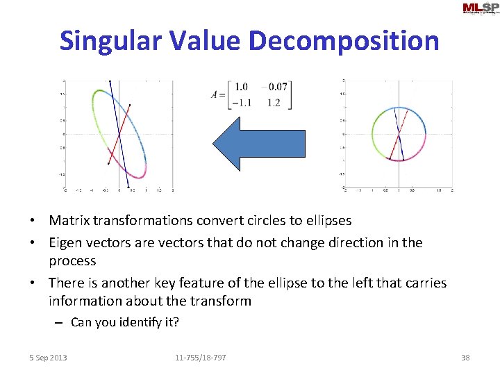
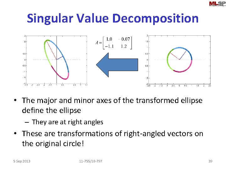
Singular Value Decomposition • Matrix transformations convert circles to ellipses • Eigen vectors are vectors that do not change direction in the process • There is another key feature of the ellipse to the left that carries information about the transform – Can you identify it? 5 Sep 2013 11 -755/18 -797 38

Singular Value Decomposition • The major and minor axes of the transformed ellipse define the ellipse – They are at right angles • These are transformations of right-angled vectors on the original circle! 5 Sep 2013 11 -755/18 -797 39

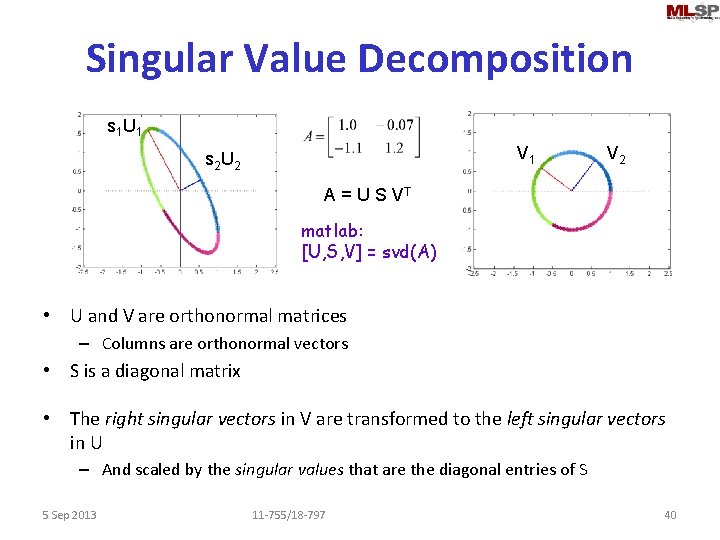
Singular Value Decomposition s 1 U 1 V 1 s 2 U 2 V 2 A = U S VT matlab: [U, S, V] = svd(A) • U and V are orthonormal matrices – Columns are orthonormal vectors • S is a diagonal matrix • The right singular vectors in V are transformed to the left singular vectors in U – And scaled by the singular values that are the diagonal entries of S 5 Sep 2013 11 -755/18 -797 40

Singular Value Decomposition • The left and right singular vectors are not the same – If A is not a square matrix, the left and right singular vectors will be of different dimensions • The singular values are always real • The largest singular value is the largest amount by which a vector is scaled by A – Max (|Ax| / |x|) = smax • The smallest singular value is the smallest amount by which a vector is scaled by A – Min (|Ax| / |x|) = smin – This can be 0 (for low-rank or non-square matrices) 5 Sep 2013 11 -755/18 -797 41

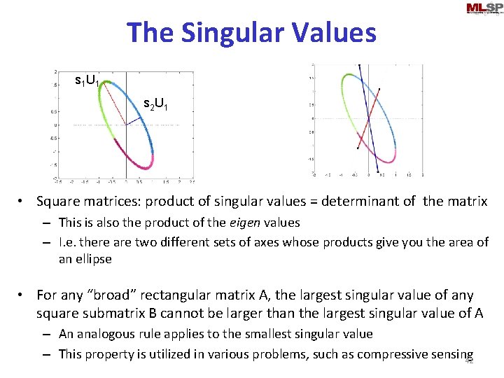
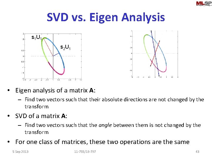
The Singular Values s 1 U 1 s 2 U 1 • Square matrices: product of singular values = determinant of the matrix – This is also the product of the eigen values – I. e. there are two different sets of axes whose products give you the area of an ellipse • For any “broad” rectangular matrix A, the largest singular value of any square submatrix B cannot be larger than the largest singular value of A – An analogous rule applies to the smallest singular value – This property is utilized in various problems, such as compressive sensing 42

SVD vs. Eigen Analysis s 1 U 1 s 2 U 1 • Eigen analysis of a matrix A: – Find two vectors such that their absolute directions are not changed by the transform • SVD of a matrix A: – Find two vectors such that the angle between them is not changed by the transform • For one class of matrices, these two operations are the same 5 Sep 2013 11 -755/18 -797 43

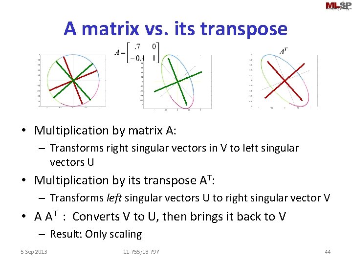
A matrix vs. its transpose • Multiplication by matrix A: – Transforms right singular vectors in V to left singular vectors U • Multiplication by its transpose AT: – Transforms left singular vectors U to right singular vector V • A AT : Converts V to U, then brings it back to V – Result: Only scaling 5 Sep 2013 11 -755/18 -797 44

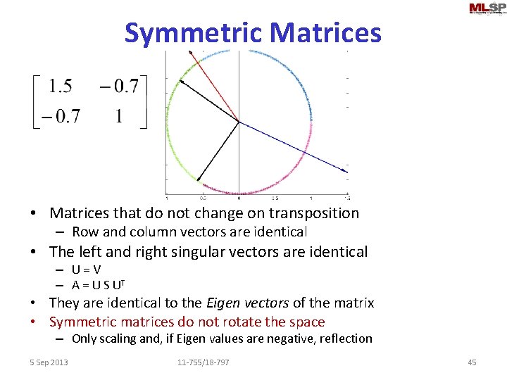
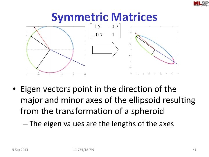
Symmetric Matrices • Matrices that do not change on transposition – Row and column vectors are identical • The left and right singular vectors are identical – U=V – A = U S UT • They are identical to the Eigen vectors of the matrix • Symmetric matrices do not rotate the space – Only scaling and, if Eigen values are negative, reflection 5 Sep 2013 11 -755/18 -797 45

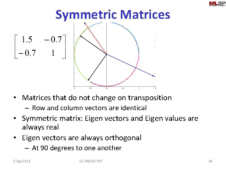
Symmetric Matrices • Matrices that do not change on transposition – Row and column vectors are identical • Symmetric matrix: Eigen vectors and Eigen values are always real • Eigen vectors are always orthogonal – At 90 degrees to one another 5 Sep 2013 11 -755/18 -797 46

Symmetric Matrices • Eigen vectors point in the direction of the major and minor axes of the ellipsoid resulting from the transformation of a spheroid – The eigen values are the lengths of the axes 5 Sep 2013 11 -755/18 -797 47

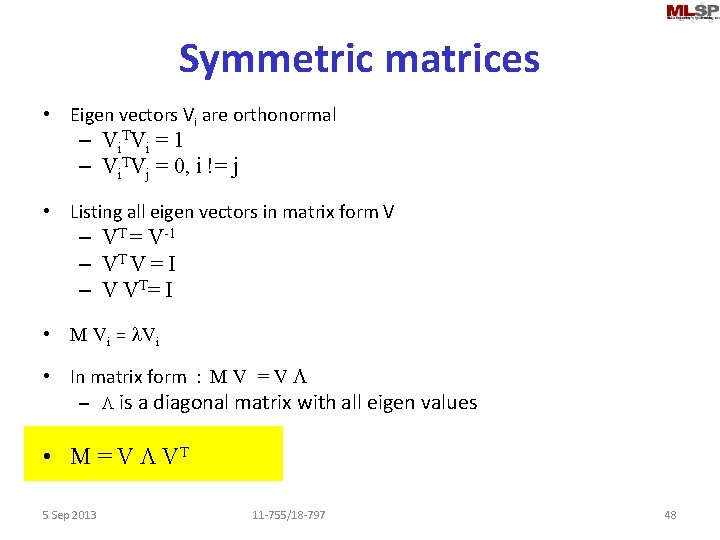
Symmetric matrices • Eigen vectors Vi are orthonormal – Vi T Vi = 1 – Vi. TVj = 0, i != j • Listing all eigen vectors in matrix form V – VT = V-1 – VT V = I – V VT = I • M Vi = l. Vi • In matrix form : M V = V L – L is a diagonal matrix with all eigen values • M = V L VT 5 Sep 2013 11 -755/18 -797 48

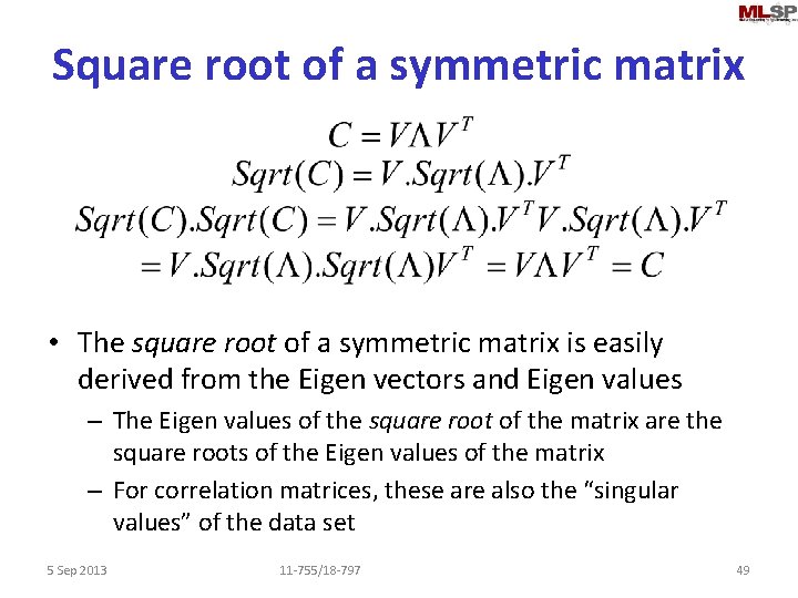
Square root of a symmetric matrix • The square root of a symmetric matrix is easily derived from the Eigen vectors and Eigen values – The Eigen values of the square root of the matrix are the square roots of the Eigen values of the matrix – For correlation matrices, these are also the “singular values” of the data set 5 Sep 2013 11 -755/18 -797 49

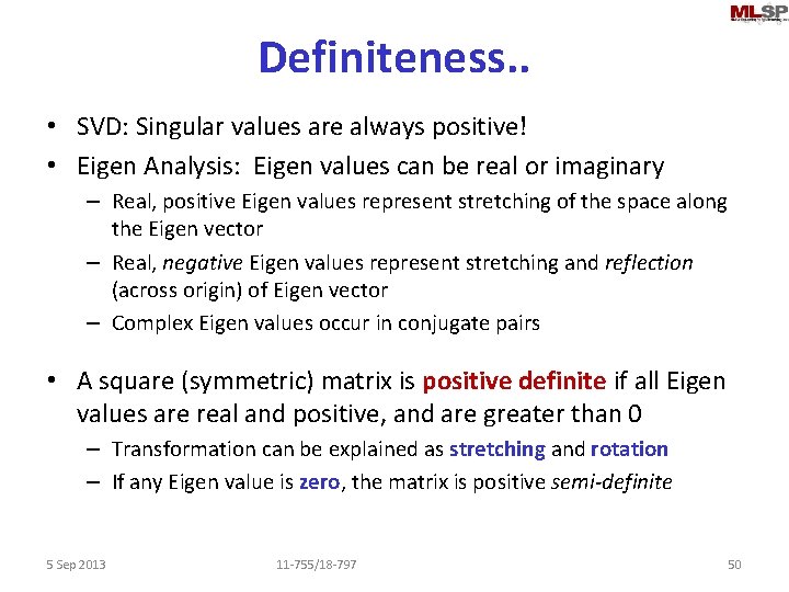
Definiteness. . • SVD: Singular values are always positive! • Eigen Analysis: Eigen values can be real or imaginary – Real, positive Eigen values represent stretching of the space along the Eigen vector – Real, negative Eigen values represent stretching and reflection (across origin) of Eigen vector – Complex Eigen values occur in conjugate pairs • A square (symmetric) matrix is positive definite if all Eigen values are real and positive, and are greater than 0 – Transformation can be explained as stretching and rotation – If any Eigen value is zero, the matrix is positive semi-definite 5 Sep 2013 11 -755/18 -797 50

Positive Definiteness. . • Property of a positive definite matrix: Defines inner product norms – x. TAx is always positive for any vector x if A is positive definite • Positive definiteness is a test for validity of Gram matrices – Such as correlation and covariance matrices – We will encounter other gram matrices later 5 Sep 2013 11 -755/18 -797 51

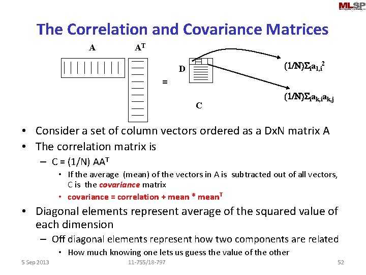
The Correlation and Covariance Matrices A AT (1/N)Sia 1, i 2 D = C (1/N)Siak, j • Consider a set of column vectors ordered as a Dx. N matrix A • The correlation matrix is – C = (1/N) AAT • If the average (mean) of the vectors in A is subtracted out of all vectors, C is the covariance matrix • covariance = correlation + mean * mean. T • Diagonal elements represent average of the squared value of each dimension – Off diagonal elements represent how two components are related • How much knowing one lets us guess the value of the other 5 Sep 2013 11 -755/18 -797 52

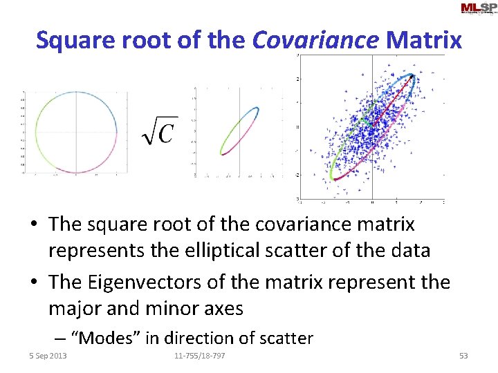
Square root of the Covariance Matrix • The square root of the covariance matrix represents the elliptical scatter of the data • The Eigenvectors of the matrix represent the major and minor axes – “Modes” in direction of scatter 5 Sep 2013 11 -755/18 -797 53

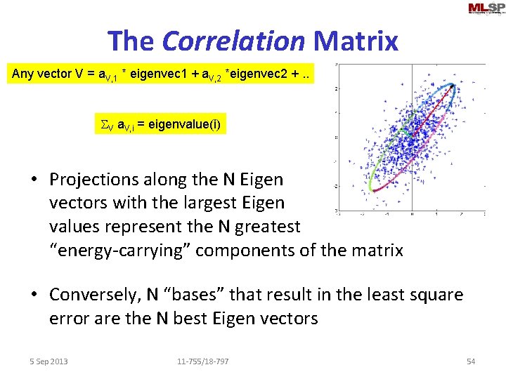
The Correlation Matrix Any vector V = a. V, 1 * eigenvec 1 + a. V, 2 *eigenvec 2 +. . SV a. V, i = eigenvalue(i) • Projections along the N Eigen vectors with the largest Eigen values represent the N greatest “energy-carrying” components of the matrix • Conversely, N “bases” that result in the least square error are the N best Eigen vectors 5 Sep 2013 11 -755/18 -797 54

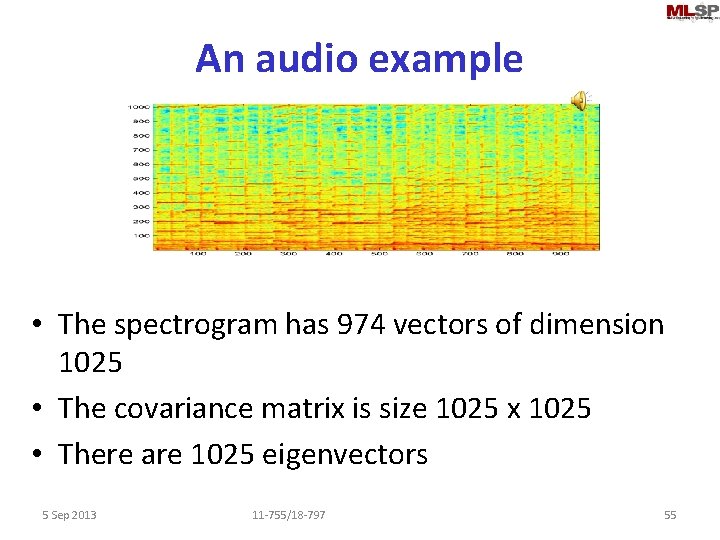
An audio example • The spectrogram has 974 vectors of dimension 1025 • The covariance matrix is size 1025 x 1025 • There are 1025 eigenvectors 5 Sep 2013 11 -755/18 -797 55

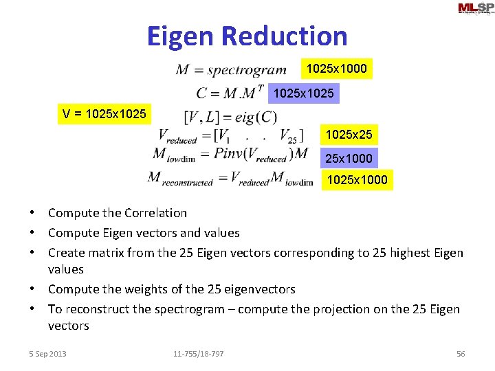
Eigen Reduction 1025 x 1000 1025 x 1025 V = 1025 x 25 25 x 1000 1025 x 1000 • Compute the Correlation • Compute Eigen vectors and values • Create matrix from the 25 Eigen vectors corresponding to 25 highest Eigen values • Compute the weights of the 25 eigenvectors • To reconstruct the spectrogram – compute the projection on the 25 Eigen vectors 5 Sep 2013 11 -755/18 -797 56

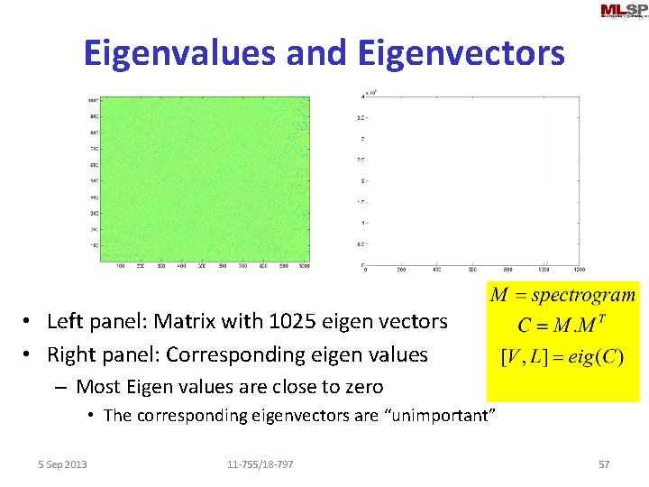
Eigenvalues and Eigenvectors • Left panel: Matrix with 1025 eigen vectors • Right panel: Corresponding eigen values – Most Eigen values are close to zero • The corresponding eigenvectors are “unimportant” 5 Sep 2013 11 -755/18 -797 57

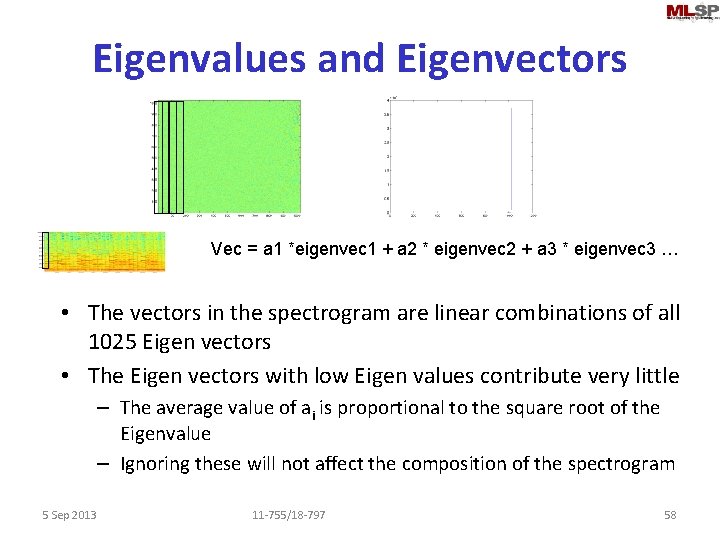
Eigenvalues and Eigenvectors Vec = a 1 *eigenvec 1 + a 2 * eigenvec 2 + a 3 * eigenvec 3 … • The vectors in the spectrogram are linear combinations of all 1025 Eigen vectors • The Eigen vectors with low Eigen values contribute very little – The average value of ai is proportional to the square root of the Eigenvalue – Ignoring these will not affect the composition of the spectrogram 5 Sep 2013 11 -755/18 -797 58

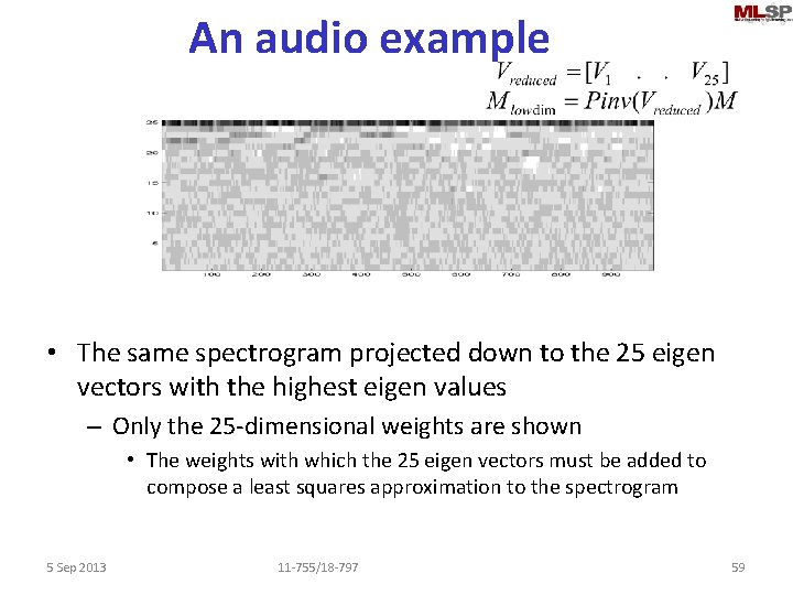
An audio example • The same spectrogram projected down to the 25 eigen vectors with the highest eigen values – Only the 25 -dimensional weights are shown • The weights with which the 25 eigen vectors must be added to compose a least squares approximation to the spectrogram 5 Sep 2013 11 -755/18 -797 59

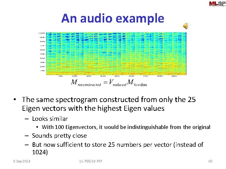
An audio example • The same spectrogram constructed from only the 25 Eigen vectors with the highest Eigen values – Looks similar • With 100 Eigenvectors, it would be indistinguishable from the original – Sounds pretty close – But now sufficient to store 25 numbers per vector (instead of 1024) 5 Sep 2013 11 -755/18 -797 60

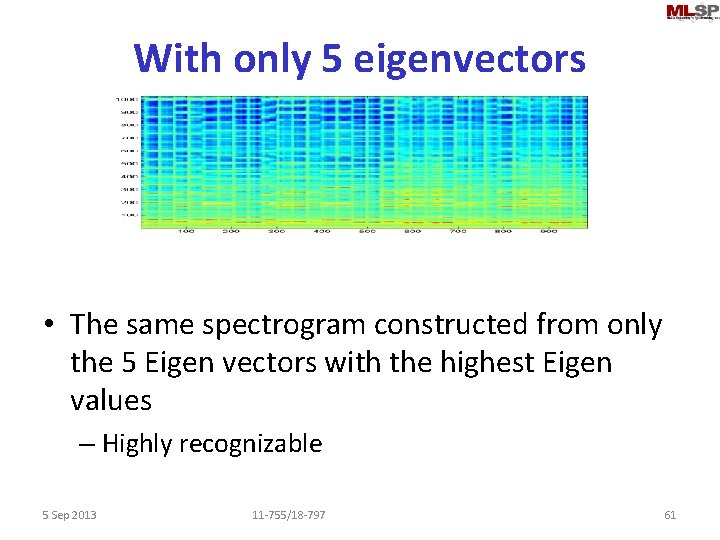
With only 5 eigenvectors • The same spectrogram constructed from only the 5 Eigen vectors with the highest Eigen values – Highly recognizable 5 Sep 2013 11 -755/18 -797 61

Correlation vs. Covariance Matrix • Correlation: – The N Eigen vectors with the largest Eigen values represent the N greatest “energy-carrying” components of the matrix – Conversely, N “bases” that result in the least square error are the N best Eigen vectors • Projections onto these Eigen vectors retain the most energy • Covariance: – the N Eigen vectors with the largest Eigen values represent the N greatest “variance-carrying” components of the matrix – Conversely, N “bases” that retain the maximum possible variance are the N best Eigen vectors 5 Sep 2013 11 -755/18 -797 62

Eigenvectors, Eigenvalues and Covariances/Correlations • The eigenvectors and eigenvalues (singular values) derived from the correlation matrix are important • Do we need to actually compute the correlation matrix? – No • Direct computation using Singular Value Decomposition 5 Sep 2013 11 -755/18 -797 63

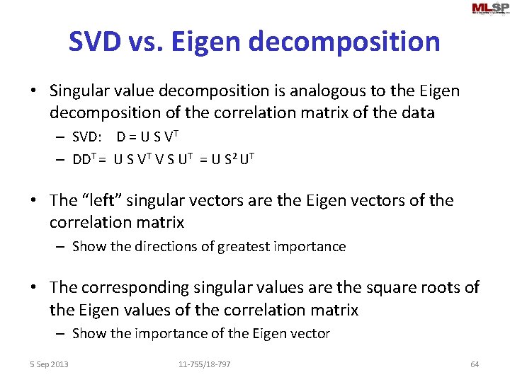
SVD vs. Eigen decomposition • Singular value decomposition is analogous to the Eigen decomposition of the correlation matrix of the data – SVD: D = U S VT – DDT = U S VT V S UT = U S 2 UT • The “left” singular vectors are the Eigen vectors of the correlation matrix – Show the directions of greatest importance • The corresponding singular values are the square roots of the Eigen values of the correlation matrix – Show the importance of the Eigen vector 5 Sep 2013 11 -755/18 -797 64

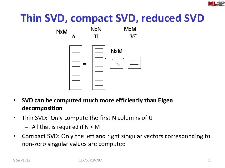
Thin SVD, compact SVD, reduced SVD Nx. M Nx. N U A Mx. M VT . Nx. M . = • SVD can be computed much more efficiently than Eigen decomposition • Thin SVD: Only compute the first N columns of U – All that is required if N < M • Compact SVD: Only the left and right singular vectors corresponding to non-zero singular values are computed 5 Sep 2013 11 -755/18 -797 65

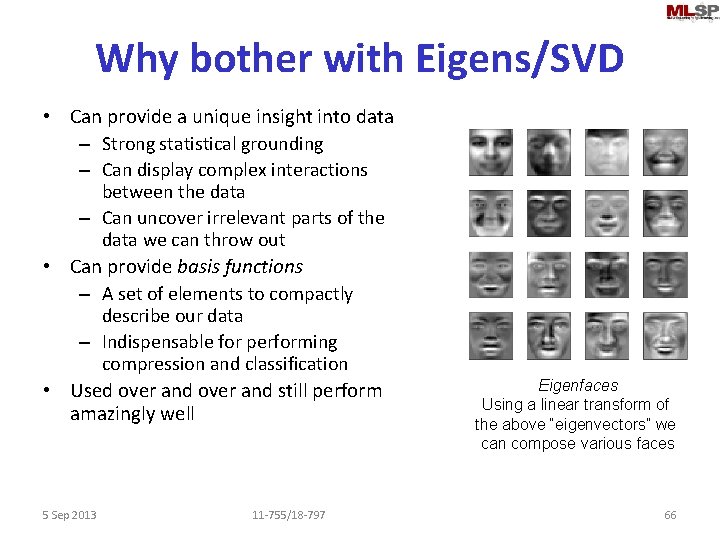
Why bother with Eigens/SVD • Can provide a unique insight into data – Strong statistical grounding – Can display complex interactions between the data – Can uncover irrelevant parts of the data we can throw out • Can provide basis functions – A set of elements to compactly describe our data – Indispensable for performing compression and classification • Used over and still perform amazingly well 5 Sep 2013 11 -755/18 -797 Eigenfaces Using a linear transform of the above “eigenvectors” we can compose various faces 66

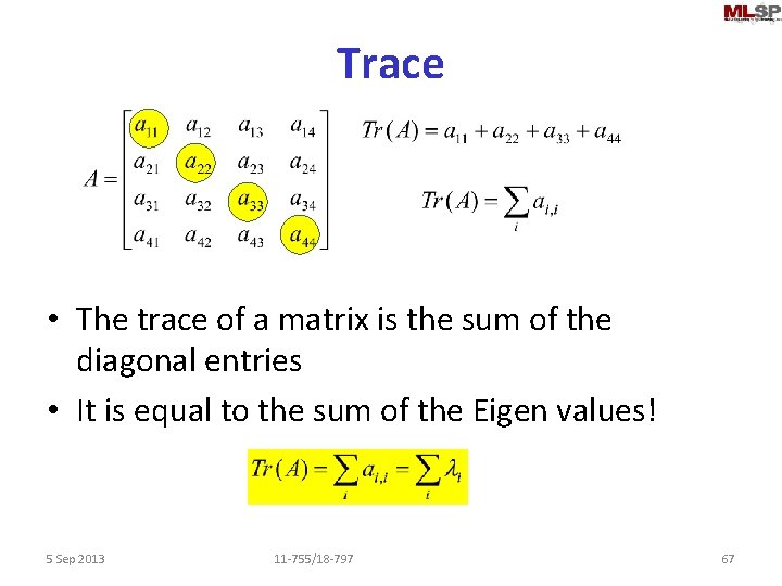
Trace • The trace of a matrix is the sum of the diagonal entries • It is equal to the sum of the Eigen values! 5 Sep 2013 11 -755/18 -797 67

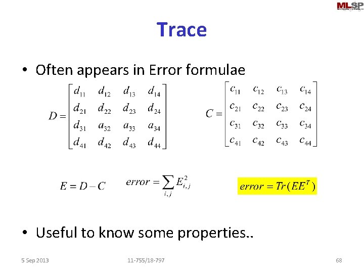
Trace • Often appears in Error formulae • Useful to know some properties. . 5 Sep 2013 11 -755/18 -797 68

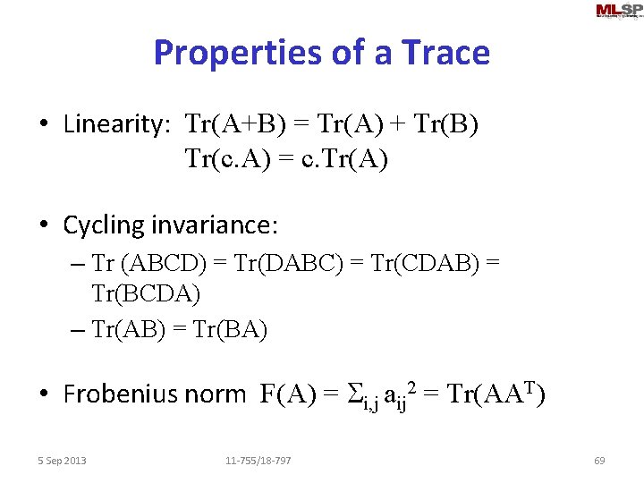
Properties of a Trace • Linearity: Tr(A+B) = Tr(A) + Tr(B) Tr(c. A) = c. Tr(A) • Cycling invariance: – Tr (ABCD) = Tr(DABC) = Tr(CDAB) = Tr(BCDA) – Tr(AB) = Tr(BA) • Frobenius norm F(A) = Si, j aij 2 = Tr(AAT) 5 Sep 2013 11 -755/18 -797 69

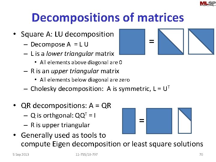
Decompositions of matrices • Square A: LU decomposition = – Decompose A = L U – L is a lower triangular matrix • All elements above diagonal are 0 – R is an upper triangular matrix • All elements below diagonal are zero – Cholesky decomposition: A is symmetric, L = UT • QR decompositions: A = QR – Q is orthgonal: QQT = I – R is upper triangular = • Generally used as tools to compute Eigen decomposition or least square solutions 5 Sep 2013 11 -755/18 -797 70

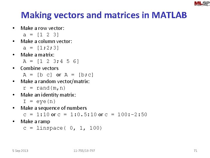
Making vectors and matrices in MATLAB • • Make a row vector: a = [1 2 3] Make a column vector: a = [1; 2; 3] Make a matrix: A = [1 2 3; 4 5 6] Combine vectors A = [b c] or A = [b; c] Make a random vector/matrix: r = rand(m, n) Make an identity matrix: I = eye(n) Make a sequence of numbers c = 1: 10 or c = 1: 0. 5: 10 or c = 100: -2: 50 Make a ramp c = linspace( 0, 1, 100) 5 Sep 2013 11 -755/18 -797 71

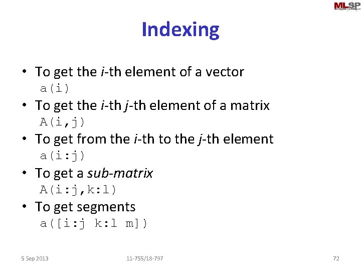
Indexing • To get the i-th element of a vector a(i) • To get the i-th j-th element of a matrix A(i, j) • To get from the i-th to the j-th element a(i: j) • To get a sub-matrix A(i: j, k: l) • To get segments a([i: j k: l m]) 5 Sep 2013 11 -755/18 -797 72

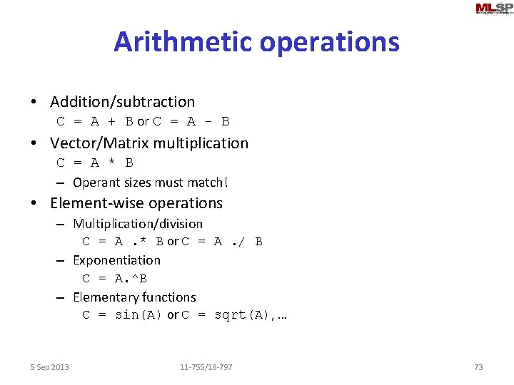
Arithmetic operations • Addition/subtraction C = A + B or C = A - B • Vector/Matrix multiplication C = A * B – Operant sizes must match! • Element-wise operations – Multiplication/division C = A. * B or C = A. / B – Exponentiation C = A. ^B – Elementary functions C = sin(A) or C = sqrt(A), … 5 Sep 2013 11 -755/18 -797 73

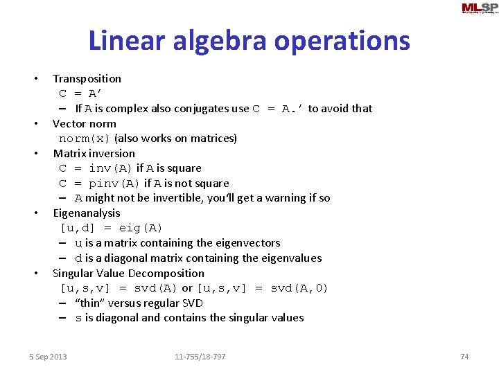
Linear algebra operations • • • Transposition C = A’ – If A is complex also conjugates use C = A. ’ to avoid that Vector norm(x) (also works on matrices) Matrix inversion C = inv(A) if A is square C = pinv(A) if A is not square – A might not be invertible, you‘ll get a warning if so Eigenanalysis [u, d] = eig(A) – u is a matrix containing the eigenvectors – d is a diagonal matrix containing the eigenvalues Singular Value Decomposition [u, s, v] = svd(A) or [u, s, v] = svd(A, 0) – “thin” versus regular SVD – s is diagonal and contains the singular values 5 Sep 2013 11 -755/18 -797 74

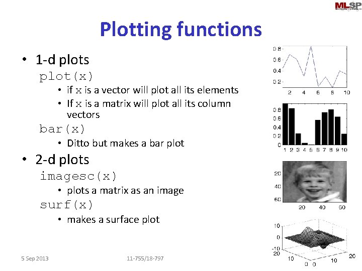
Plotting functions • 1 -d plots plot(x) • if x is a vector will plot all its elements • If x is a matrix will plot all its column vectors bar(x) • Ditto but makes a bar plot • 2 -d plots imagesc(x) • plots a matrix as an image surf(x) • makes a surface plot 5 Sep 2013 11 -755/18 -797 75

Getting help with functions • The help function – Type help followed by a function name • Things to try help help help + eig svd plot bar imagesc surf ops matfun • Also check out the tutorials and the mathworks site 5 Sep 2013 11 -755/18 -797 76