Local Field Potentials Spikes and Modeling Strategies for

Local Field Potentials, Spikes and Modeling Strategies for Both Robert Haslinger Dept. of Brain and Cog. Sciences: MIT Martinos Center for Biomedical Imaging: MGH

Outline 1. 2. 3. 4. Extra-cellular electric potentials, their origin, and their filtering Local Field Potential and Continuous Models Spikes and Generalized Linear Models Example of GLM modeling in rat barrel cortex

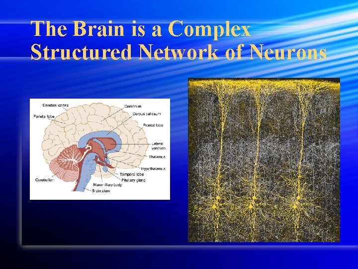
The Brain is a Complex Structured Network of Neurons

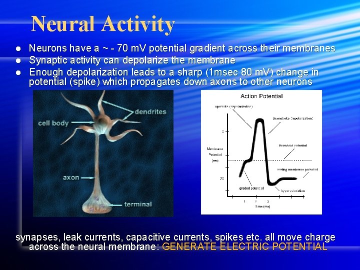
Neural Activity l l l Neurons have a ~ - 70 m. V potential gradient across their membranes Synaptic activity can depolarize the membrane Enough depolarization leads to a sharp (1 msec 80 m. V) change in potential (spike) which propagates down axons to other neurons synapses, leak currents, capacitive currents, spikes etc. all move charge across the neural membrane: GENERATE ELECTRIC POTENTIAL

What do we actually measure ?

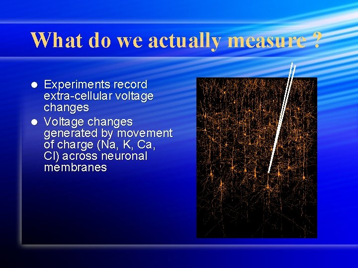
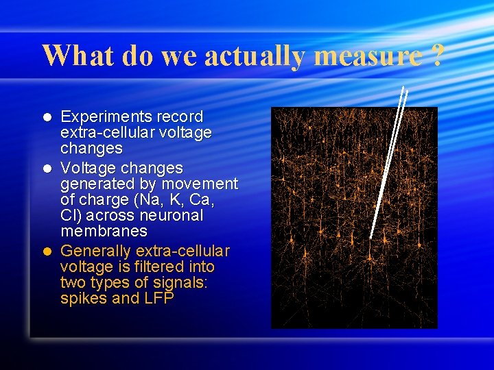
What do we actually measure ? Experiments record extra-cellular voltage changes l Voltage changes generated by movement of charge (Na, K, Ca, Cl) across neuronal membranes l

What do we actually measure ? Experiments record extra-cellular voltage changes l Voltage changes generated by movement of charge (Na, K, Ca, Cl) across neuronal membranes l Generally extra-cellular voltage is filtered into two types of signals: spikes and LFP l

Local Field Potential

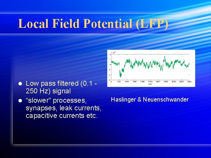
Local Field Potential (LFP) Low pass filtered (0. 1 250 Hz) signal l “slower” processes, synapses, leak currents, capacitive currents etc. l Haslinger & Neuenschwander

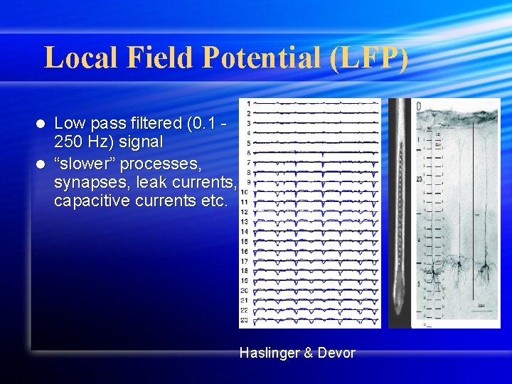
Local Field Potential (LFP) Low pass filtered (0. 1 250 Hz) signal l “slower” processes, synapses, leak currents, capacitive currents etc. l Haslinger & Devor

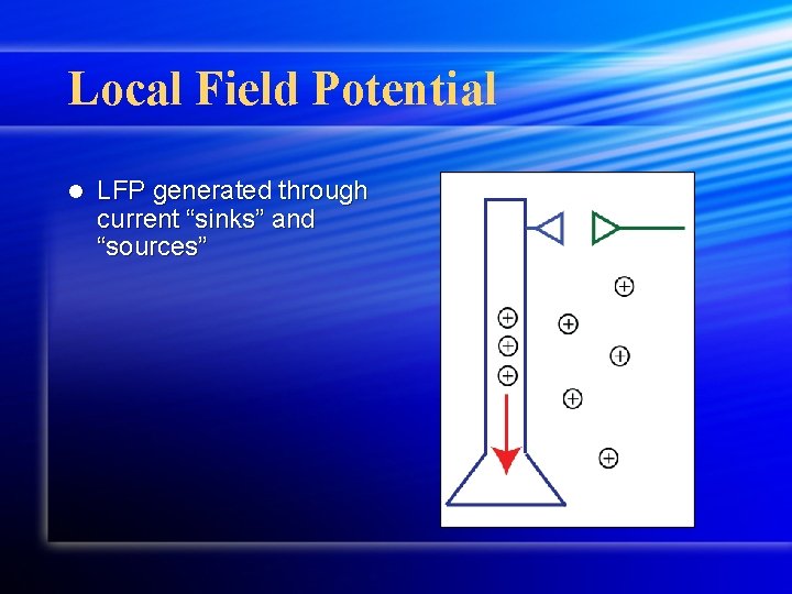
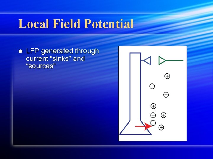
Local Field Potential l LFP generated through current “sinks” and “sources”

Local Field Potential l LFP generated through current “sinks” and “sources”

Local Field Potential l LFP generated through current “sinks” and “sources”

Local Field Potential l LFP generated through current “sinks” and “sources”

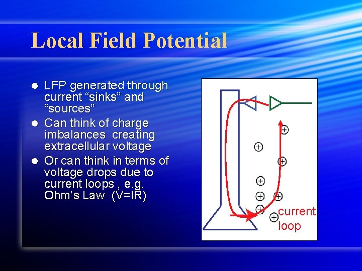
Local Field Potential LFP generated through current “sinks” and “sources” l Can think of charge imbalances creating extracellular voltage l

Local Field Potential LFP generated through current “sinks” and “sources” l Can think of charge imbalances creating extracellular voltage l Or can think in terms of voltage drops due to current loops , e. g. Ohm’s Law (V=IR) l current loop

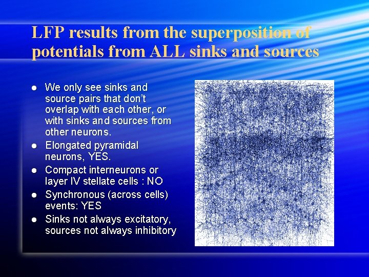
LFP results from the superposition of potentials from ALL sinks and sources l l l We only see sinks and source pairs that don’t overlap with each other, or with sinks and sources from other neurons. Elongated pyramidal neurons, YES. Compact interneurons or layer IV stellate cells : NO Synchronous (across cells) events: YES Sinks not always excitatory, sources not always inhibitory

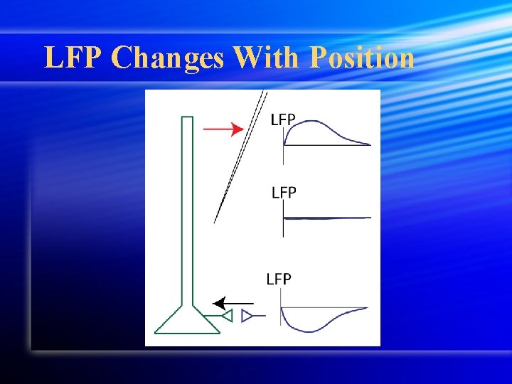
LFP Changes With Position

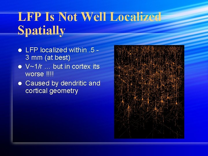
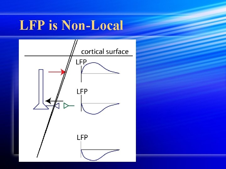
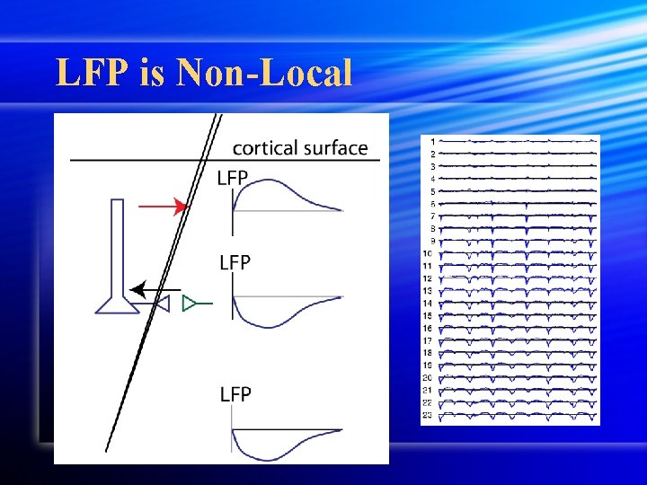
LFP Is Not Well Localized Spatially LFP localized within. 5 3 mm (at best) l V~1/r … but in cortex its worse !!!! l Caused by dendritic and cortical geometry l

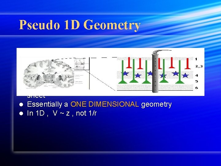
Pseudo 1 D Geometry Cortex is a thin (2 -3 mm thick) sheet Greatest anatomical variation perpendicular to the sheet l Essentially a ONE DIMENSIONAL geometry l In 1 D , V ~ z , not 1/r l l

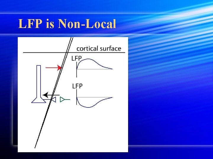
LFP is Non-Local

LFP is Non-Local

LFP is Non-Local

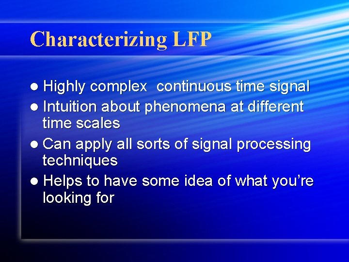
Characterizing LFP l Highly complex continuous time signal l Intuition about phenomena at different time scales l Can apply all sorts of signal processing techniques l Helps to have some idea of what you’re looking for

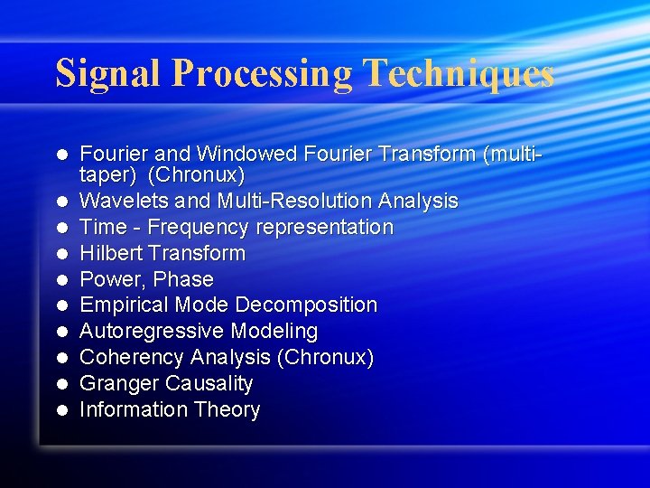
Signal Processing Techniques l l l l l Fourier and Windowed Fourier Transform (multitaper) (Chronux) Wavelets and Multi-Resolution Analysis Time - Frequency representation Hilbert Transform Power, Phase Empirical Mode Decomposition Autoregressive Modeling Coherency Analysis (Chronux) Granger Causality Information Theory

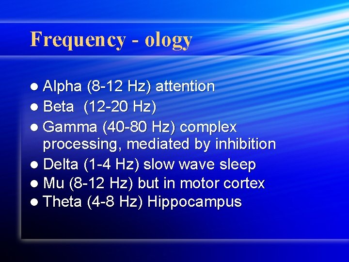
Frequency - ology l Alpha (8 -12 Hz) attention l Beta (12 -20 Hz) l Gamma (40 -80 Hz) complex processing, mediated by inhibition l Delta (1 -4 Hz) slow wave sleep l Mu (8 -12 Hz) but in motor cortex l Theta (4 -8 Hz) Hippocampus

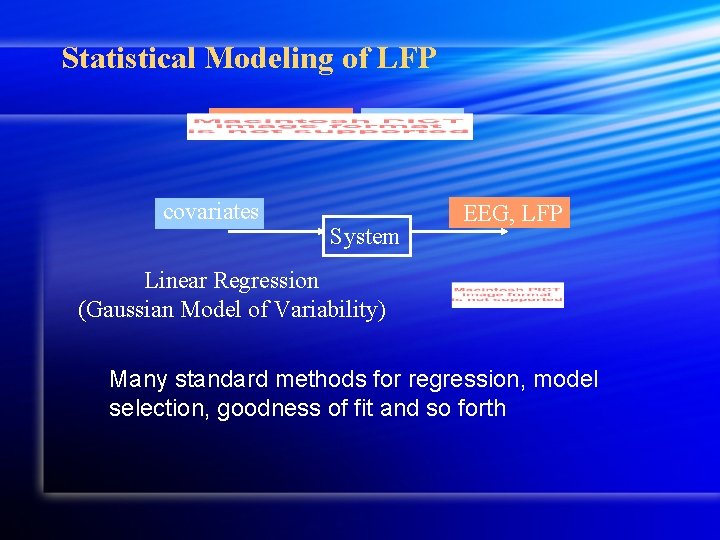
Statistical Modeling of LFP covariates System EEG, LFP Linear Regression (Gaussian Model of Variability) Many standard methods for regression, model selection, goodness of fit and so forth

Spikes

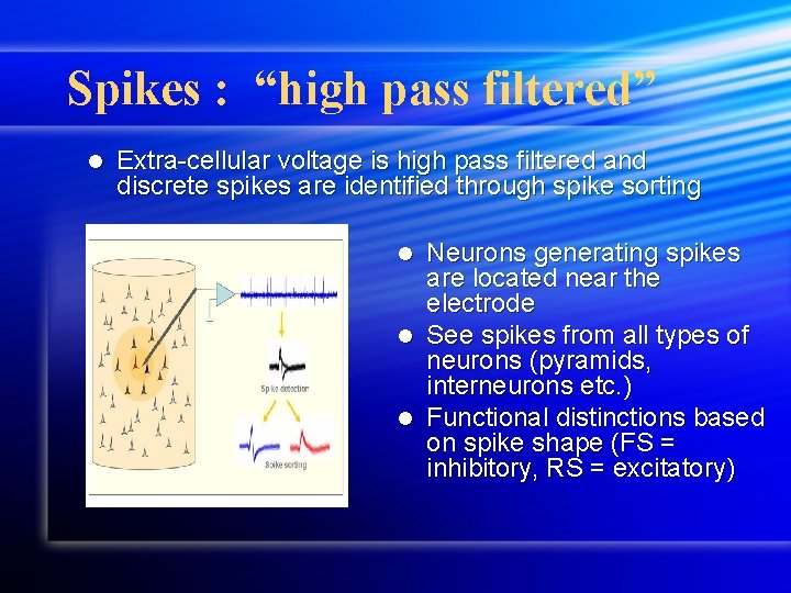
Spikes : “high pass filtered” l Extra-cellular voltage is high pass filtered and discrete spikes are identified through spike sorting Neurons generating spikes are located near the electrode l See spikes from all types of neurons (pyramids, interneurons etc. ) l Functional distinctions based on spike shape (FS = inhibitory, RS = excitatory) l

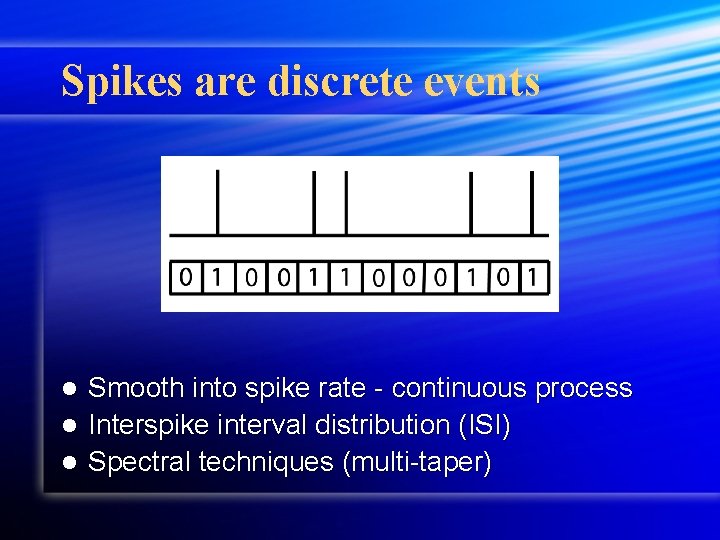
Spikes are discrete events Smooth into spike rate - continuous process l Interspike interval distribution (ISI) l Spectral techniques (multi-taper) l

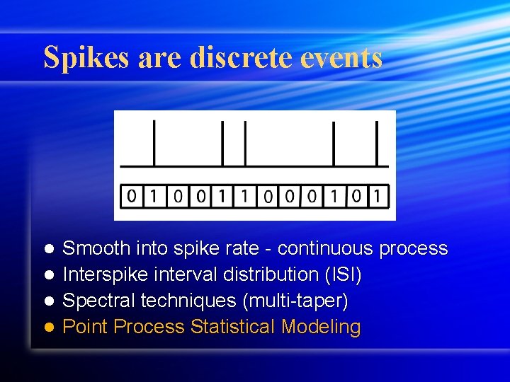
Spikes are discrete events Smooth into spike rate - continuous process l Interspike interval distribution (ISI) l Spectral techniques (multi-taper) l Point Process Statistical Modeling l

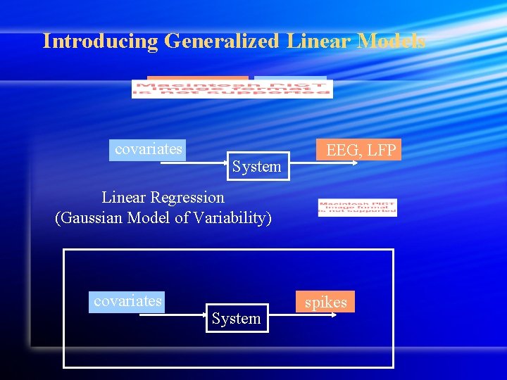
Introducing Generalized Linear Models covariates System EEG, LFP Linear Regression (Gaussian Model of Variability) covariates System spikes

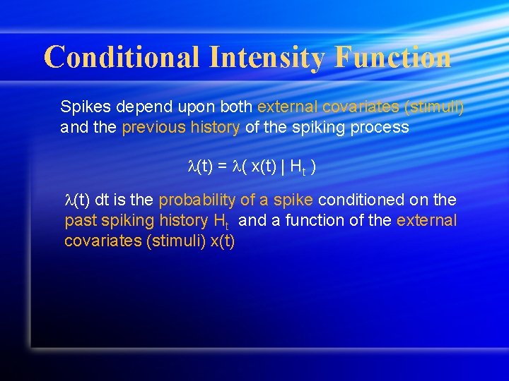
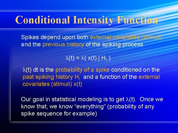
Conditional Intensity Function Spikes depend upon both external covariates (stimuli) and the previous history of the spiking process (t) = ( x(t) | Ht ) (t) dt is the probability of a spike conditioned on the past spiking history Ht and a function of the external covariates (stimuli) x(t)

Conditional Intensity Function Spikes depend upon both external covariates (stimuli) and the previous history of the spiking process (t) = ( x(t) | Ht ) (t) dt is the probability of a spike conditioned on the past spiking history Ht and a function of the external covariates (stimuli) x(t) Our goal in statistical modeling is to get (t). Once we know that, we know “everything” (probability of any spike sequence for example)

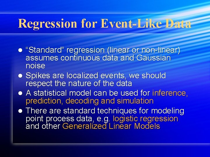
Regression for Event-Like Data “Standard” regression (linear or non-linear) assumes continuous data and Gaussian noise l Spikes are localized events, we should respect the nature of the data l A statistical model can be used for inference, prediction, decoding and simulation l There are standard techniques for modeling point process data, e. g. logistic regression and other Generalized Linear Models l

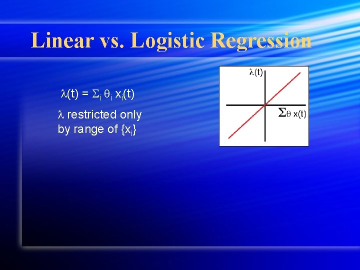
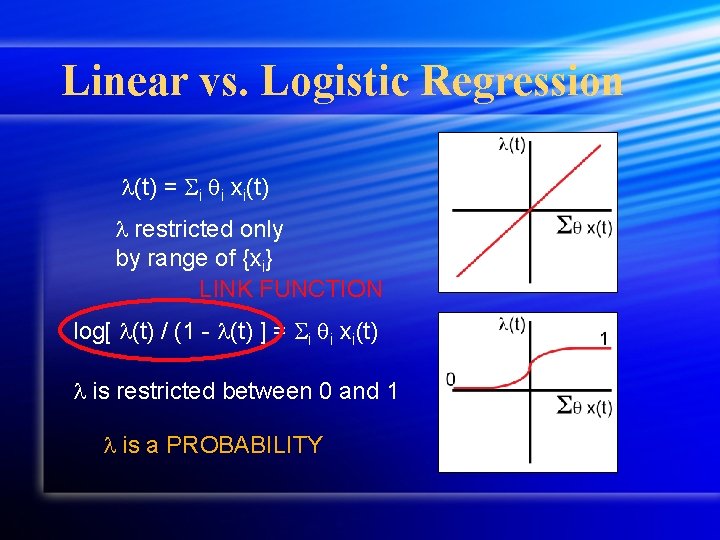
Linear vs. Logistic Regression (t) = i i xi(t) restricted only by range of {xi}

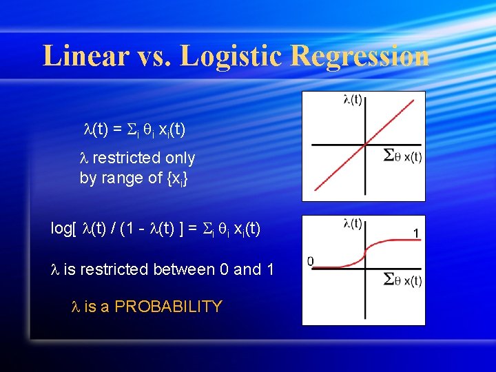
Linear vs. Logistic Regression (t) = i i xi(t) restricted only by range of {xi} log[ (t) / (1 - (t) ] = i i xi(t) is restricted between 0 and 1 is a PROBABILITY

Linear vs. Logistic Regression (t) = i i xi(t) restricted only by range of {xi} LINK FUNCTION log[ (t) / (1 - (t) ] = i i xi(t) is restricted between 0 and 1 is a PROBABILITY

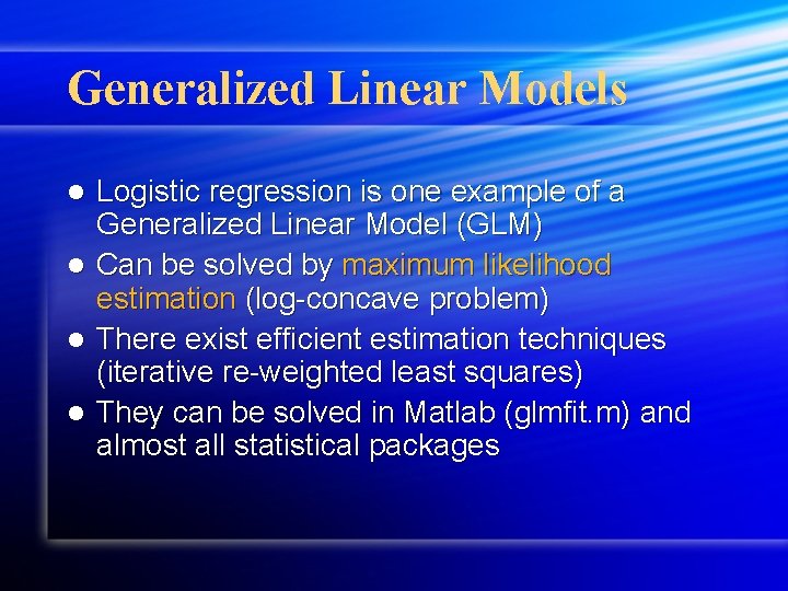
Generalized Linear Models l l Logistic regression is one example of a Generalized Linear Model (GLM) Can be solved by maximum likelihood estimation (log-concave problem) There exist efficient estimation techniques (iterative re-weighted least squares) They can be solved in Matlab (glmfit. m) and almost all statistical packages

Possible Covariates to Include log[ (t) / (1 - (t)) ] = i i fi (stimulus)

Possible Covariates to Include log[ (t) / (1 - (t)) ] = i i fi (stimulus) j j gj (spiking history)

Possible Covariates to Include log[ (t) / (1 - (t)) ] = i i fi (stimulus) j j gj (spiking history) k k hk (ensemble spiking)

Possible Covariates to Include log[ (t) / (1 - (t)) ] = i i fi (stimulus) j j gj (spiking history) k k hk (ensemble spiking) p p rp (LFP)

Possible Covariates to Include log[ (t) / (1 - (t)) ] = i i fi (stimulus) j j gj (spiking history) k k hk (ensemble spiking) p p rp (LFP) Fitted parameters give the importance of different contributions

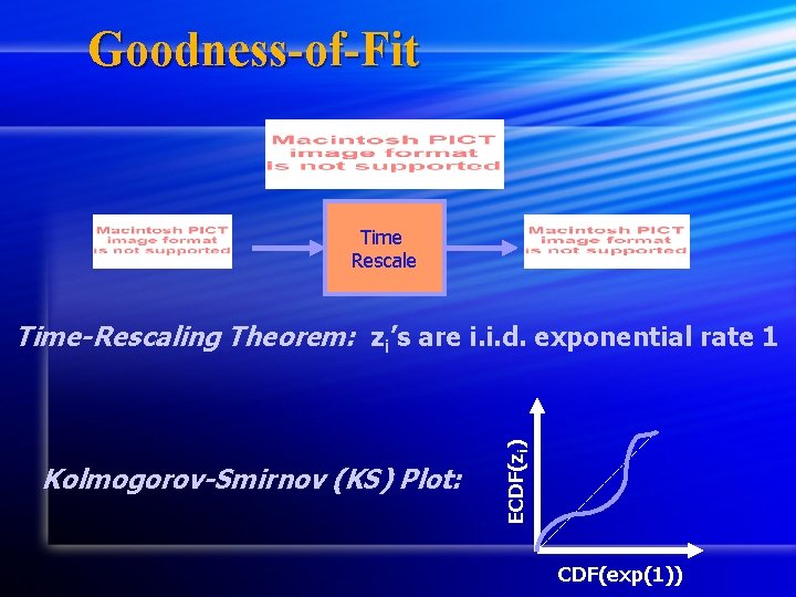
Goodness-of-Fit Time Rescale Kolmogorov-Smirnov (KS) Plot: ECDF(zi) Time-Rescaling Theorem: zi’s are i. i. d. exponential rate 1 CDF(exp(1))

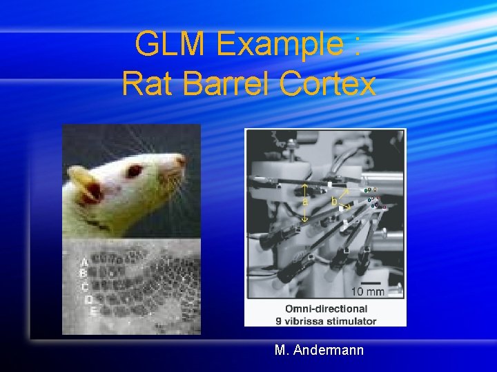
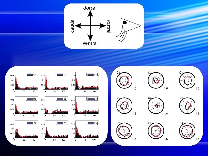
GLM Example : Rat Barrel Cortex M. Andermann

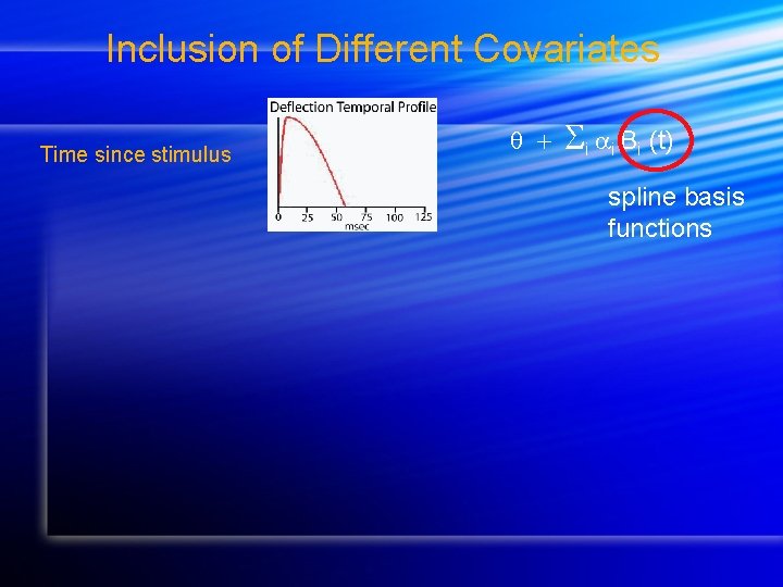
Inclusion of Different Covariates

Inclusion of Different Covariates Time since stimulus i i Bi (t) spline basis functions

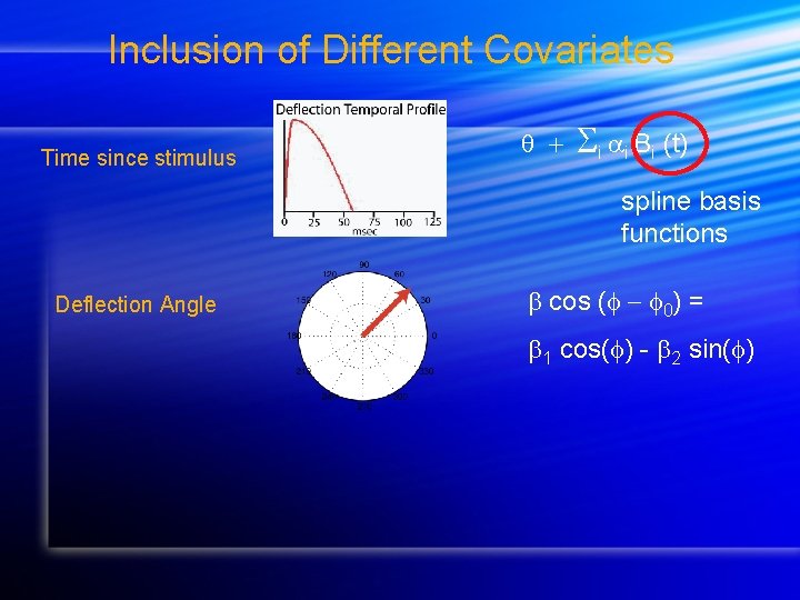
Inclusion of Different Covariates Time since stimulus i i Bi (t) spline basis functions Deflection Angle cos ( 0) = 1 cos( ) - 2 sin( )

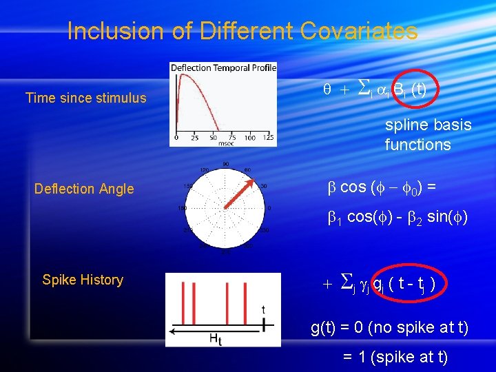
Inclusion of Different Covariates Time since stimulus i i Bi (t) spline basis functions Deflection Angle cos ( 0) = 1 cos( ) - 2 sin( ) Spike History j j gj ( t - tj ) g(t) = 0 (no spike at t) = 1 (spike at t)

FINAL MODEL log[ (t) / (1 - (t) ) ] = i i Bi (t) + 1 cos( ) - 2 sin( ) j j gj ( t - tj )

FINAL MODEL log[ (t) / (1 - (t) ) ] = i i Bi (t) + 1 cos( ) - 2 sin( ) j j gj ( t - tj ) Often spike history effects account for most of the statistics !!!!!!! History Term

FINAL MODEL log[ (t) / (1 - (t) ) ] = i i Bi (t) + 1 cos( ) - 2 sin( ) j j gj ( t - tj ) Often spike history effects account for most of the statistics !!!!!!! History Term bursting refractory

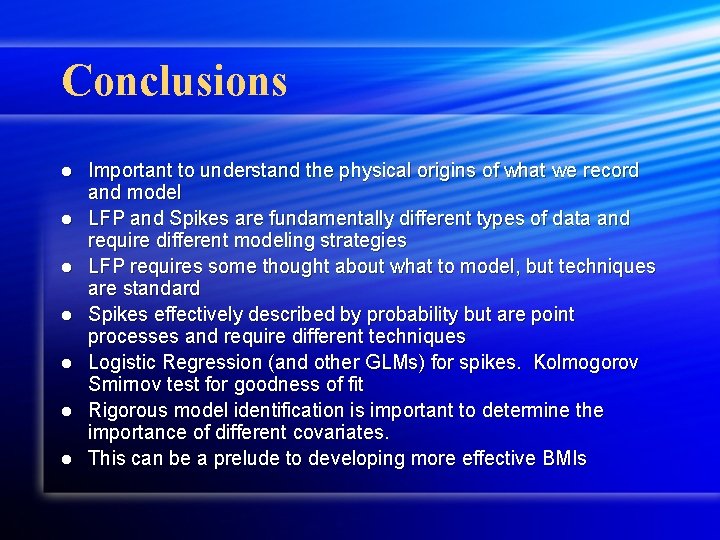
Conclusions l l l l Important to understand the physical origins of what we record and model LFP and Spikes are fundamentally different types of data and require different modeling strategies LFP requires some thought about what to model, but techniques are standard Spikes effectively described by probability but are point processes and require different techniques Logistic Regression (and other GLMs) for spikes. Kolmogorov Smirnov test for goodness of fit Rigorous model identification is important to determine the importance of different covariates. This can be a prelude to developing more effective BMIs