The retarded potentials LL 2 Section 62 Potentials

 in")
 Equation for potentials of arbitrary field")


 1 D wave equation")


 Note that")

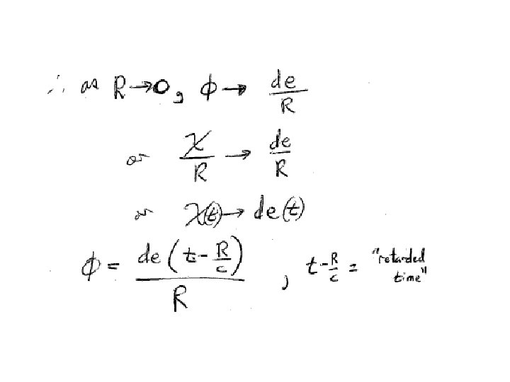
 for")

- Slides: 17
The retarded potentials LL 2 Section 62
Potentials for arbitrarily moving charges 2 nd pair of Maxwell’s equations (30. 2) in 4 -D
Choose the Lorentz gauge (46. 9) Equation for potentials of arbitrary field
3 D form Space Components: Time Components: If fields are constant, we get Poisson equations (36. 4) & (43. 4) If there are no charges, we get the homogeneous wave equation (46. 7) d’Alembertian operator
Solution to inhomogeneous equation = solution to homogeneous equation + particular solution Recipe 1. Divide space into infinitesimal volume elements 2. Find field due to charges in each element 3. The total field is the linear superposition of the fields from all elements
Field point Source point de is generally time dependent.
Put the origin inside d. V. Then… Field point
Equation for the scalar potential Everywhere but at the origin we have The problem is centrally symmetric
Use spherical coordinates Away from the origin Trial solution (HW) 1 D wave equation
Solutions to the 1 D wave equation are of the form Allow outgoing waves only Substitute this combination of R and t into the trial solution (Holds everywhere except the origin. )
Now determine c to match the potential at the origin Df increases more rapidly than as R goes to zero. Neglect the time derivative We already know the solution to this from Coulomb’s law (36. 9)
For an arbitrary distribution of charge, set de = r d. V and integrate Retarded time Particular solution Solution to the homogeneous equation
Field point r is evaluated at the Shorthand expression retarded time t-(R/c) Note that the integration variable r’ is buried in R in two places. Prime omitted
Same method for vector potential Retarded potential Solution of homogeneous equation
If charges are stationary, scalar potential should reduce to usual result (36. 8) for constant E-field + f 0 If currents are stationary, vector potential should reduce to usual result (43. 5) for constant H-field + A 0 <A>t =
Homogeneous solutions f 0 and A 0 are determined by initial conditions or by constant boundary conditions Example: Scattering Scattered radiation is determined by retarded potentials Incident radiation from outside is determined by f 0 and A 0