Electromagnetic Potentials E f Scalar Potential f and

- Slides: 25
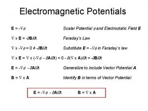
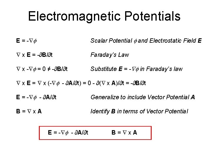
Electromagnetic Potentials E = - f Scalar Potential f and Electrostatic Field E x E = -∂B/∂t Faraday’s Law x - f = 0 ≠ -∂B/∂t Substitute E = - f in Faraday’s law x E = x (- f - ∂A/∂t) = 0 - ∂( x A)/∂t = -∂B/∂t E = - f - ∂A/∂t Generalize to include Vector Potential A B= x. A Identify B in terms of Vector Potential E = - f - ∂A/∂t B= x. A
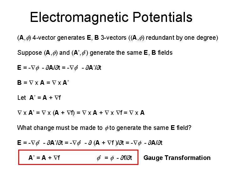
Electromagnetic Potentials (A, f) 4 -vector generates E, B 3 -vectors ((A, f) redundant by one degree) Suppose (A, f) and (A’, f’) generate the same E, B fields E = - f - ∂A/∂t = - f’ - ∂A’/∂t B = x A’ Let A’ = A + f x A’ = x (A + f) = x A + x f = x A What change must be made to f to generate the same E field? E = - f’ - ∂A’/∂t = - f’ - ∂ (A + f )/∂t = - f - ∂A/∂t A’ = A + f f’ = f - ∂f/∂t Gauge Transformation
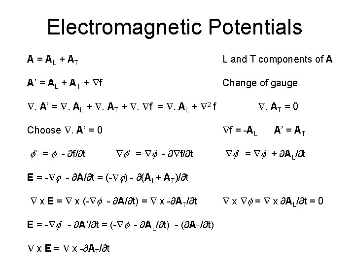
Electromagnetic Potentials A = AL + AT L and T components of A A’ = AL + AT + f Change of gauge . A’ = . AL + . AT + . f = . AL + 2 f Choose . A’ = 0 f’ = f - ∂f/∂t . AT = 0 f = -AL f’ = f - ∂ f/∂t A’ = AT f’ = f + ∂AL/∂t E = - f - ∂A/∂t = (- f) - ∂(AL+ AT)/∂t x E = x (- f - ∂A/∂t) = x -∂AT/∂t E = - f’ - ∂A’/∂t = (- f - ∂AL/∂t) - (∂AT/∂t) x E = x -∂AT/∂t x f = x ∂AL/∂t = 0
Electromagnetic Potentials
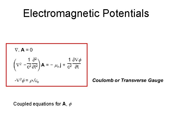
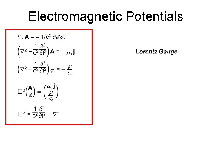
Electromagnetic Potentials Coupled equations for A, f
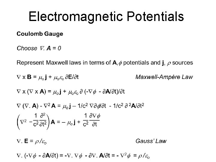
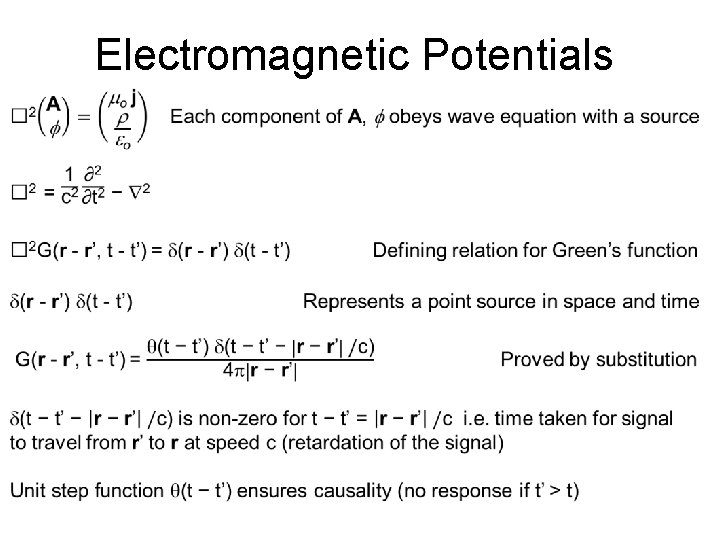
Electromagnetic Potentials
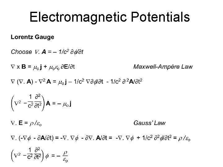
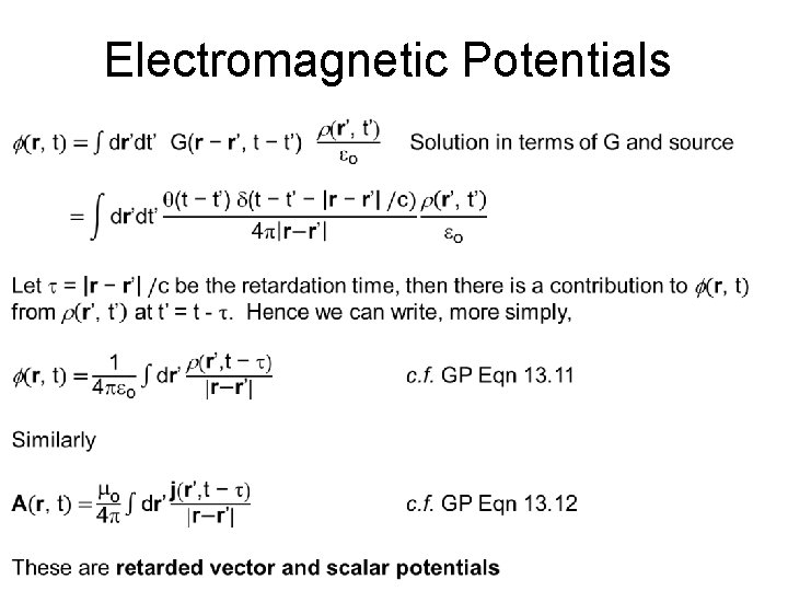
Electromagnetic Potentials
Electromagnetic Potentials
Electromagnetic Potentials
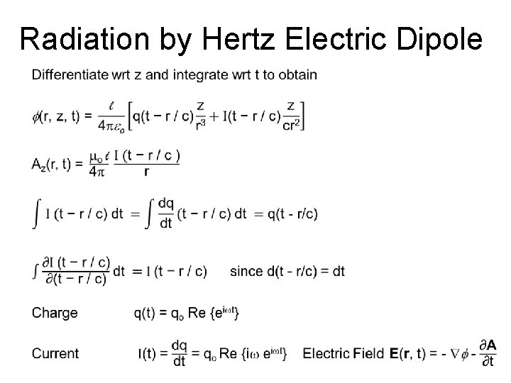
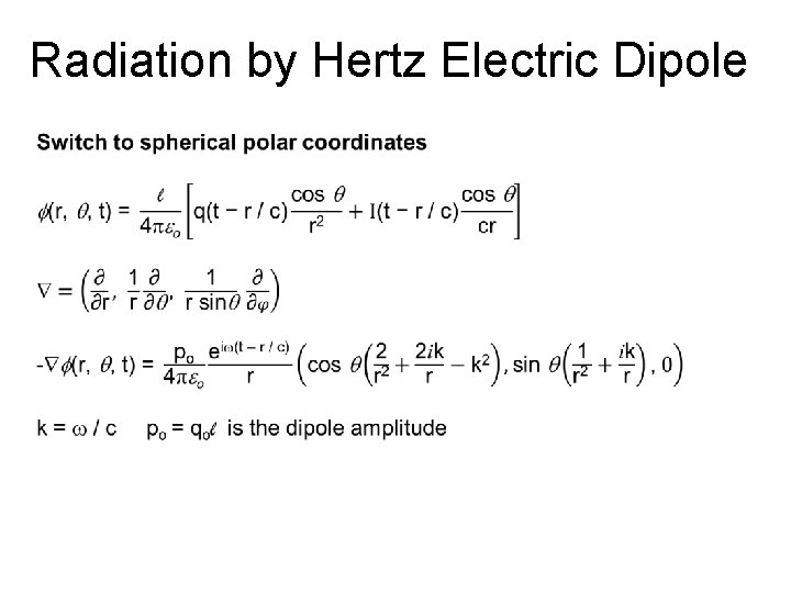
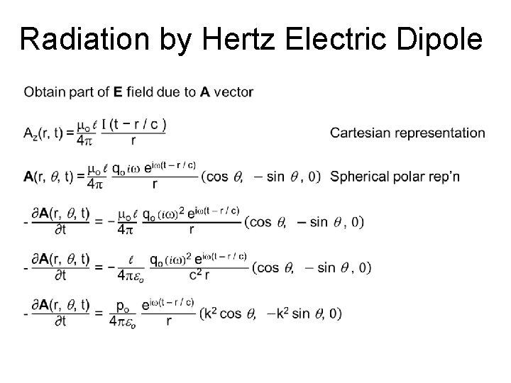
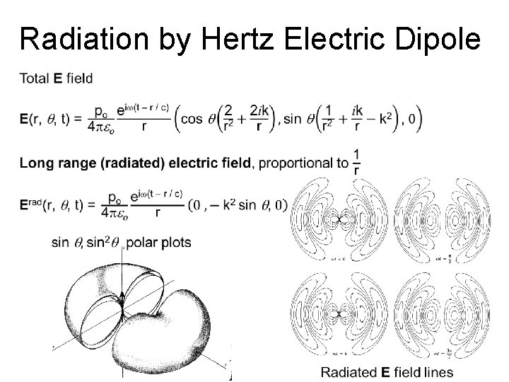
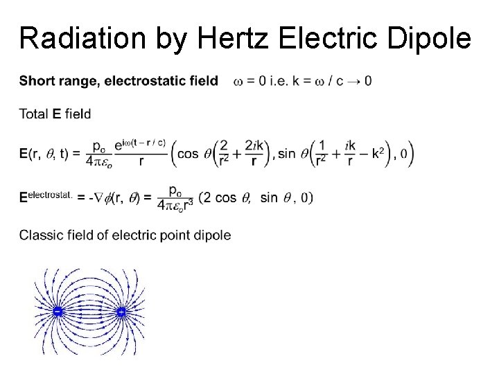
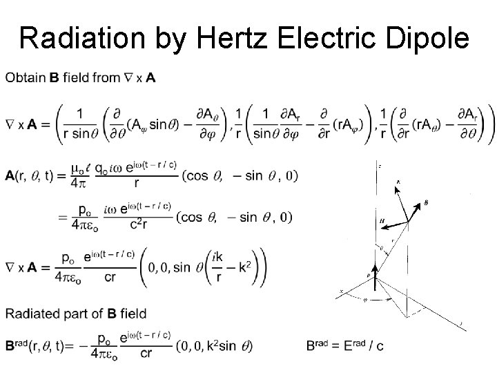
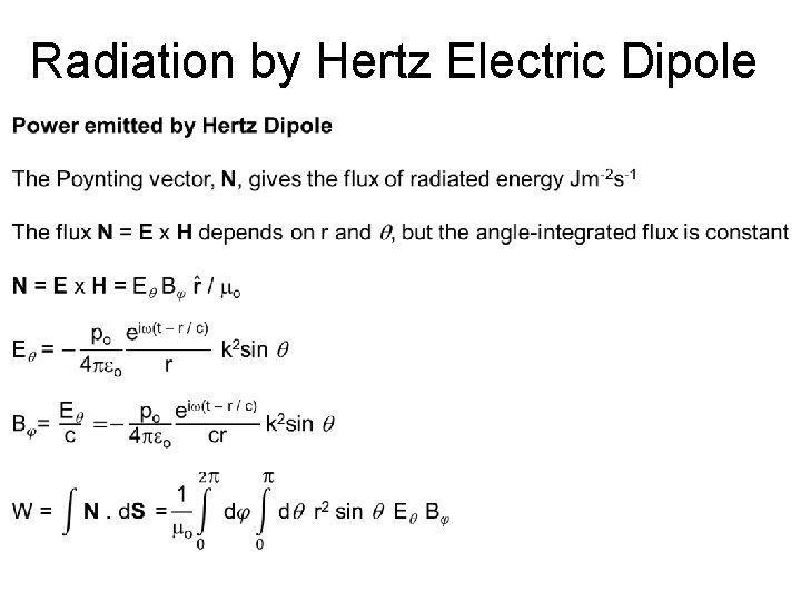
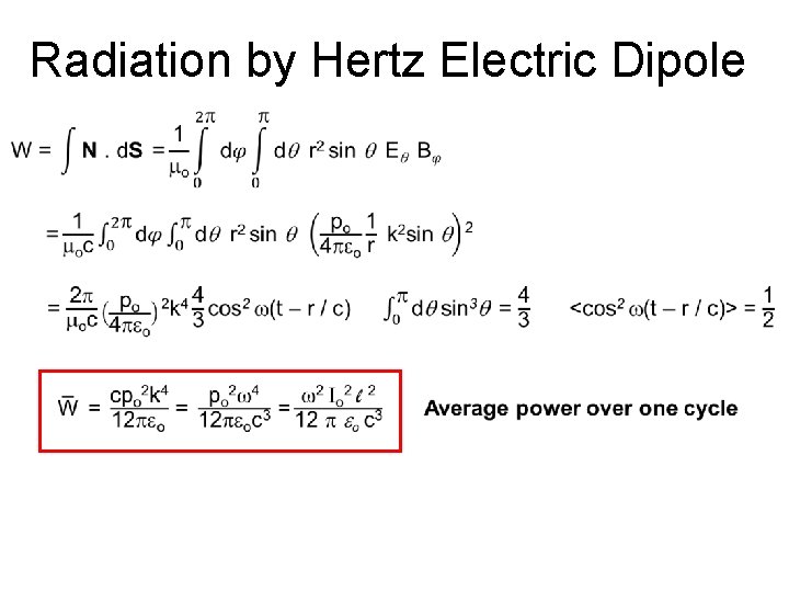
Radiation by Hertz Electric Dipole r = (x, y, z) Field Point z +q Using retarded potentials, calculate E(r, t), B(r, t) for dipole at origin y l x r' = (0, 0, z’) Source Point -q Charge Current Dipole Moment Wire Radius Current Density q(t) = qo Re {eiwt} I(t) = dq/dt = qo Re {iw eiwt} p(t) = po Re {eiwt} = qo l Re {eiwt} a j(t) = I(t) / p a 2
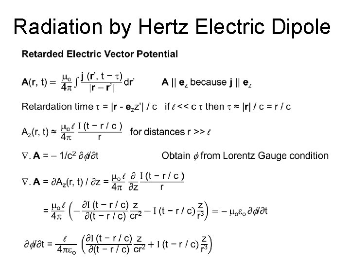
Radiation by Hertz Electric Dipole
Radiation by Hertz Electric Dipole
Radiation by Hertz Electric Dipole
Radiation by Hertz Electric Dipole
Radiation by Hertz Electric Dipole
Radiation by Hertz Electric Dipole
Radiation by Hertz Electric Dipole
Radiation by Hertz Electric Dipole
Radiation by Hertz Electric Dipole
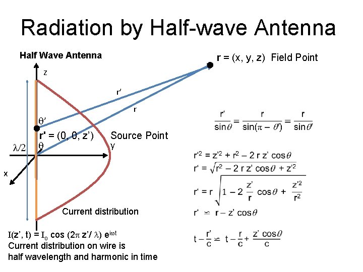
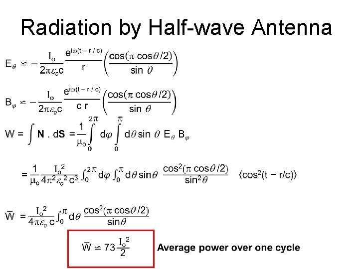
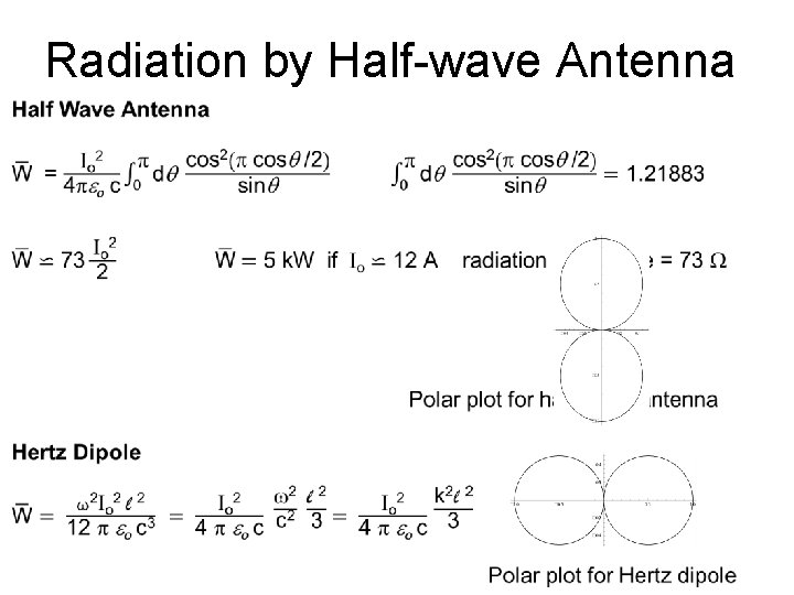
Radiation by Half-wave Antenna Half Wave Antenna r = (x, y, z) Field Point z r’ l/2 q’ r' = (0, 0, z’) q r Source Point y x Current distribution I(z’, t) = Io cos (2 p z’/ l) eiwt Current distribution on wire is half wavelength and harmonic in time
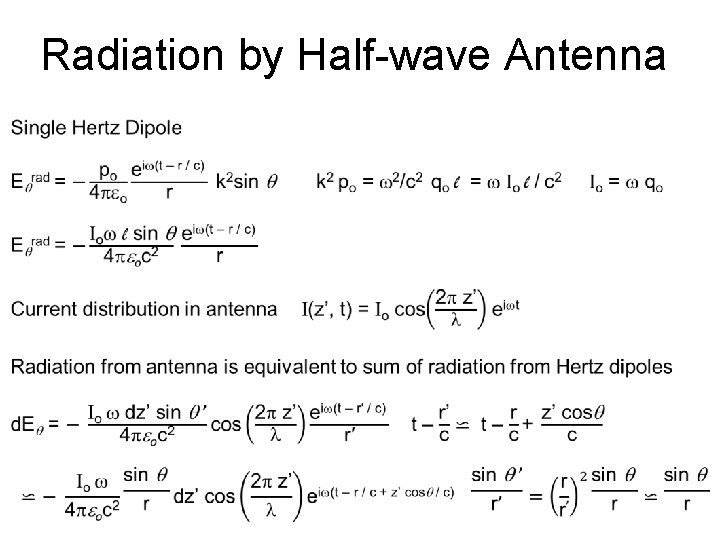
Radiation by Half-wave Antenna
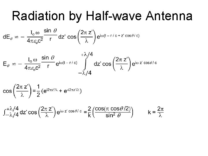
Radiation by Half-wave Antenna
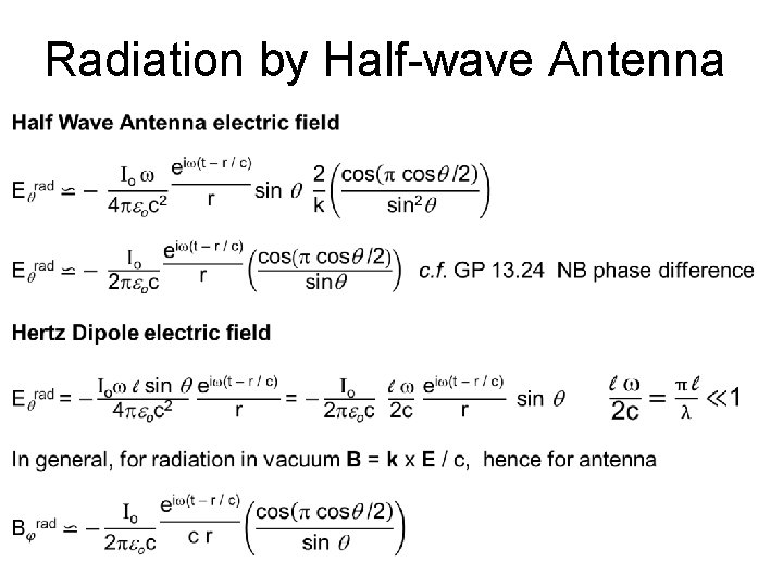
Radiation by Half-wave Antenna
Radiation by Half-wave Antenna
Radiation by Half-wave Antenna