Lecture 7 Simulations http www angelfire comlinuxlecturenotes What

Lecture 7: Simulations

http: //www. angelfire. com/linux/lecturenotes/

What will we cover in this lecture • A introduction to the idea and concept of stochastic simulation • A look at the 2 main methods of stochastic simulation: Bootstrapping & Monte Carlo Simulation • A look at the use of these methods in the calculation of risk

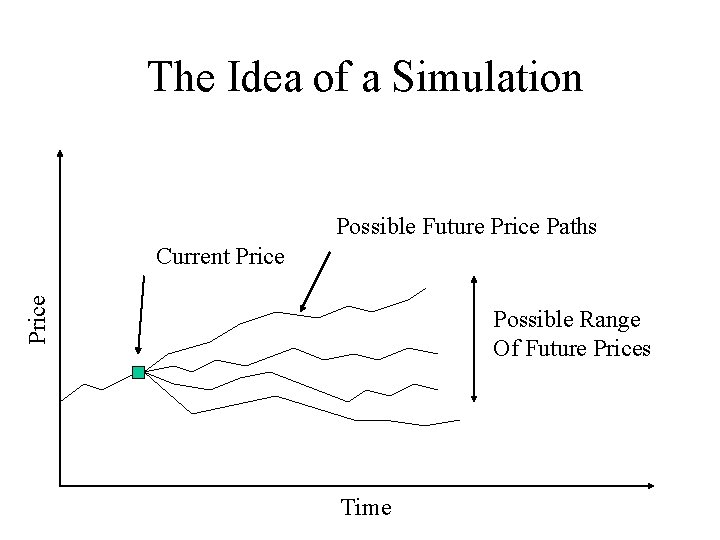
The Idea Behind Simulations • Simulations are basically the idea of simulating a set of possible future outcomes or ‘realisations’ • Each ‘future’ realisation is just one possibility of what may occur in the future • By generating many possible future realisations we can assess the range of future outcomes • In an earlier lecture we simulated a possible path for stock prices by generating a set of possible future returns from a normal distribution • This was an example of a univariate simulation (a simulation of one variable)

The Idea of a Simulation Possible Future Price Paths Price Current Price Possible Range Of Future Prices Time

Useful Simulations • For a simulation to be useful the paths generated must reflect the behaviour of the asset/liabilities we are simulating • Each randomly generated future path will then represent a ‘possible’ future outcome • The basis for both our Bootstrapping and Monte Carlo Simulations will be the Brownian Motion Process we have been using so far

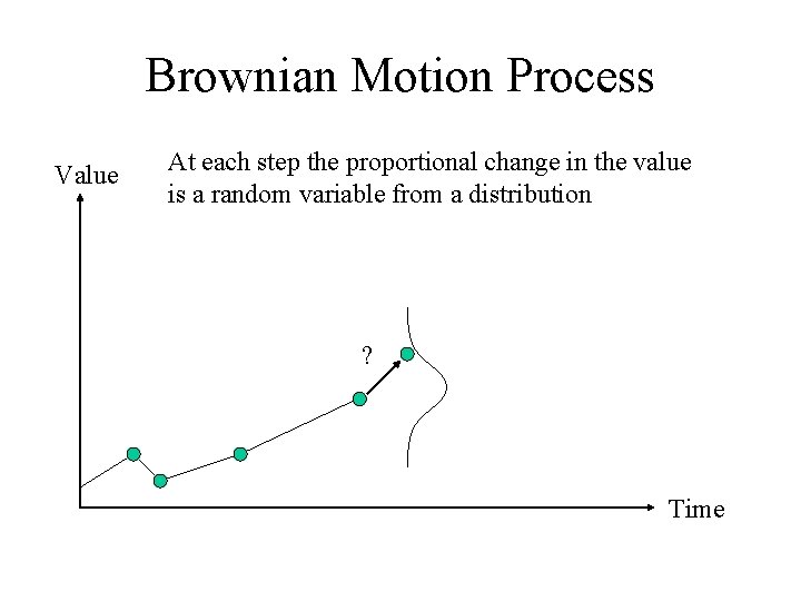
Brownian Motion Process Value At each step the proportional change in the value is a random variable from a distribution ? Time

Bootstrapping: A simple & powerful approach • Bootstrapping is based on a very simple idea: that we can use past observations as a bag from which we randomly sample to create possible future outcomes! • The premise is a simple one: all of our past observations were sampled from a given distribution and all future observations will also be sampled from this same distribution • Instead of having to estimate the underlying distribution and then sampling random variables from it we directly sample from our past observations which are representative

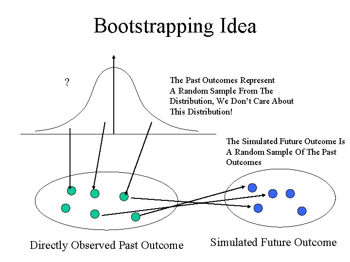
Bootstrapping Idea ? The Past Outcomes Represent A Random Sample From The Distribution, We Don’t Care About This Distribution! The Simulated Future Outcome Is A Random Sample Of The Past Outcomes Directly Observed Past Outcome Simulated Future Outcome

Univariate Bootstrap • Univariate Bootstrap is the generation of a possible path for a single simultaneous random process • We generate a pool of observations from the process’s historic behaviour • We then generate a future path by randomly sampling from this pool of observations

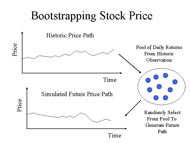
An Example: Bootstrapping a stock price • If we assume that the continuously compounded return of the stock price each day is sampled from a constant distribution then we can generate future price paths • Firstly we build up our pool of past daily returns by calculating the implied return from the price history • Secondly we randomly sample from this pool to generate a possible future path

Bootstrapping Stock Price Historic Price Path Pool of Daily Returns From Historic Observation Time Price Simulated Future Price Path Time Randomly Select From Pool To Generate Future Path

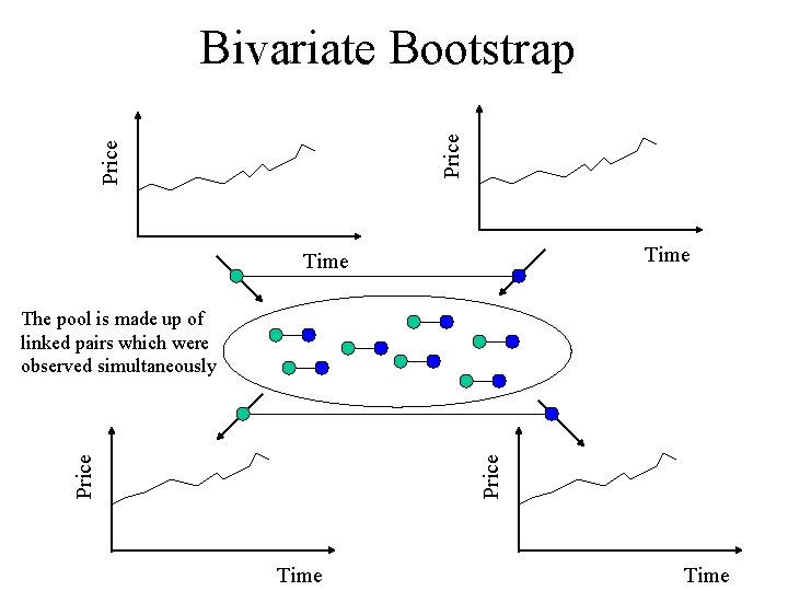
Multivariate Bootstrapping • It is equally possible to simultaneously generate future paths for multiple correlated processes • Like our univariate bootstrap we build up a pool of observations from the past • We maintain any correlations by grouping simtaneous observations together • Any correlations will be captured in these linked historic observations • When we randomly sample from the pool to generate the future paths we preserve these groupings

Price Bivariate Bootstrap Time Price The pool is made up of linked pairs which were observed simultaneously Time

What if we do not preserve the grouping of simultaneous observations? • If we do not keep the groups then we cannot expect our generated paths to reflect any correlations • If we have strong reason to believe that there is no correlation between the processes then we might break apart the observations and sample them completely randomly • We might do this to increase the size of our ‘pool’

Bootstrapping Is Very Powerful • The power of bootstrapping is that it does not rely on any statistical assumptions • All it says is that the future will be sampled from the same distribution as the past • We need a large sample of historic observations to build up a large pool • The assumption that the future will come from the same distribution as the past is crucial and requires a stationary series • This simple bootstrapping technique does not capture serial correlation across time.

Bootstrapping in Excel • For practical usage bootstrapping is better suited to a programming language such as VBA, or a specialist tool • The exercise book for this lecture contains an array function called “bootstrap” • bootstrap will take an input range and reorder it randomly • bootstrap is an array formula for which an output range must be selected and ctrl-shift-enter must be used to enter it!

Monte Carlo Simulation • The Monte Carlo Simulation generates random numbers from probability distribution rather than pools of historic observations • We will focus on Monte Carlo Simulations based about the normal distribution • We will see how we can use the Covariance matrix to generate multivariate Monte Carlo Simulations

Univariate Monte Carlo Simulations • By generating random variables sampled from a normal distribution it is possible to generate a brownian motion paths based on this sequence of random numbers • In the example of the stock price if the return is normally distributed with mean m and standard deviation s then by generating returns from a distribution with these properties we can generate a possible path for this stock • The most common method for generating normal random numbers is Box-Muller, and we will use Excel’s built in facility

Stock Price Simulation • In the case where the stock price is generated from the following process: • By generating a sequence of random variables r we can generate a future path for P • This would be an example of a univariate Monte Carlo Simulation

Price Univariate Stock Price Simulation Randomly Sampled Returns From Normal Distribution Randomly generated feasible path Time

Multivariate Monte Carlo Simulation • A multivariate Monte Carlo Simulation is where we sample random values from a multivariate distribution which captures the various correlations • So if 2 assets have a strong correlation we want to see strong correlations in the random numbers we generate • There is a set method which allows us to generate a set of ‘correlated’ normally distributed random variables using the covariance matrix

What we would like • We have described the statistical properties of returns using the expectation vector and the covariance matrix. • We would like to generate sets of random numbers that match this expected return vector and covariance matrix • We could then generate simultaneous paths for the various assets/liabilities described by these statistics

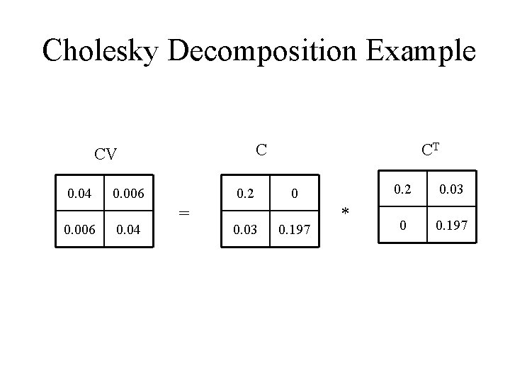
The Basis of Multivariate Monte Carlo: The Cholesky Decomposition • The Cholesky decomposition of the covariance matrix will allow us to generate sets of random variables described by the covariance matrix • The Cholesky decomposition is sometimes called the square root of a matrix • It takes the form: • Where CV is the covariance matrix and C is the cholesky decomposition. C is a lower diagonal matrix and of the same dimensions as CV • The Cholesky decomposition only exists for positive definite matrices.

Cholesky Decomposition Example C CV 0. 04 0. 006 0. 04 0. 2 = 0. 03 CT 0 0. 197 * 0. 2 0. 03 0 0. 197

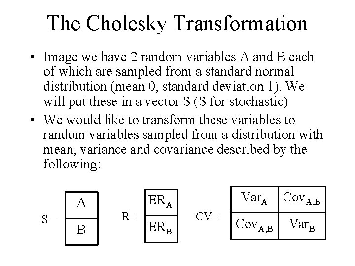
The Cholesky Transformation • Image we have 2 random variables A and B each of which are sampled from a standard normal distribution (mean 0, standard deviation 1). We will put these in a vector S (S for stochastic) • We would like to transform these variables to random variables sampled from a distribution with mean, variance and covariance described by the following: A S= B R= ERA ERB CV= Var. A Cov. A, B Var. B

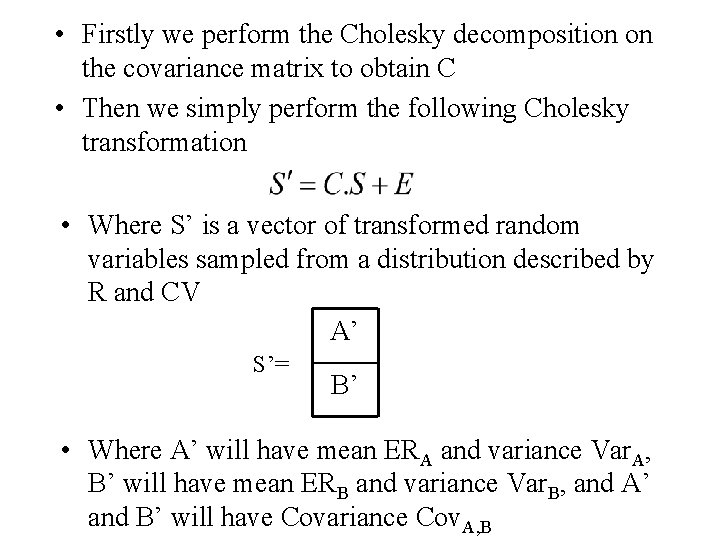
• Firstly we perform the Cholesky decomposition on the covariance matrix to obtain C • Then we simply perform the following Cholesky transformation • Where S’ is a vector of transformed random variables sampled from a distribution described by R and CV A’ S’= B’ • Where A’ will have mean ERA and variance Var. A, B’ will have mean ERB and variance Var. B, and A’ and B’ will have Covariance Cov. A, B

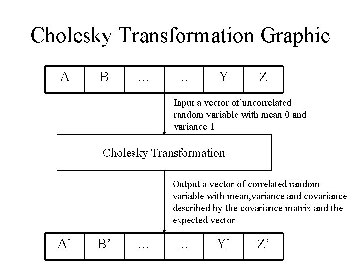
Cholesky Transformation Graphic A B … … Y Z Input a vector of uncorrelated random variable with mean 0 and variance 1 Cholesky Transformation Output a vector of correlated random variable with mean, variance and covariance described by the covariance matrix and the expected vector A’ B’ … … Y’ Z’

Cholesky Factorisations in Excel • Cholesky Factorisations are not provided by Excel’s built in matrix support • The class workbook comes with a VBA macro that will perform this factorisation for you, it is an array function called cholesky

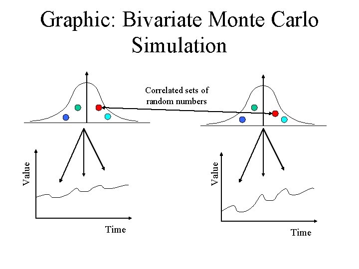
Multivariate Monte Carlo Simulation • Using the Cholesky Transformation we can generate sets of correlated random numbers • Using these sets of correlated random numbers we can generate simultaneous future paths for correlated processes • These simulated paths make up one possible future outcome in our Monte Carlo Simulation • Monte Carlo Simulations use 1000’s or even 1000000’s of possible future outcomes to build up a picture of the range of future possibilities

Graphic: Bivariate Monte Carlo Simulation Value Correlated sets of random numbers Time

General Multivariate Monte Carlo Algorithm • 1) Decompose the covariance matrix VC into its Cholesky decomposition C • 2) Generate a vector of N unit variate normal random number, where N is the dimensions of the simulation • 3) Multiply the decomposition C by the vector N to get a result vector X • 4) Add the vector X to the expected return vector R to get a vector V which contains the fully transformed random variables • 5) Add transformed vector V to the set of transformed vectors S • 6) If S contains less than the desired number of random variables then goto step 2

The montecarlo macro • Embedded in the exercise spreadsheets there is a VBA macro which runs the Monte Carlo algorithm • It take two parameters: first the range specifying the covariance matrix, second the range specifying the expected return vector • From these inputs it outputs a set of random variables sampled from a distribution described by the covariance matrix and expected vector in a range specified by the user • It is important to remember to specify one column for every random variate you want to generate and press ctrl-shift-enter to tell the computer it is an array formula!

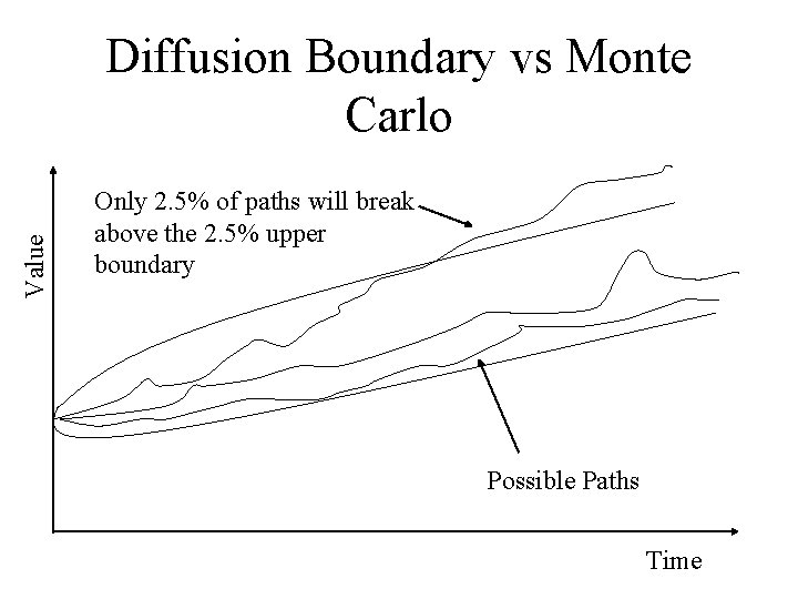
Stochastic Boundaries And Monte Carlo Simulations • In early lectures we looked at placing boundaries on the behaviour of a stochastic process • These boundaries are linked to Monte Carlo Simulations in that we expect only 5% or 2. 5% of simulations to be outside the respective diffusion boundary

Value Diffusion Boundary vs Monte Carlo Only 2. 5% of paths will break above the 2. 5% upper boundary Possible Paths Time

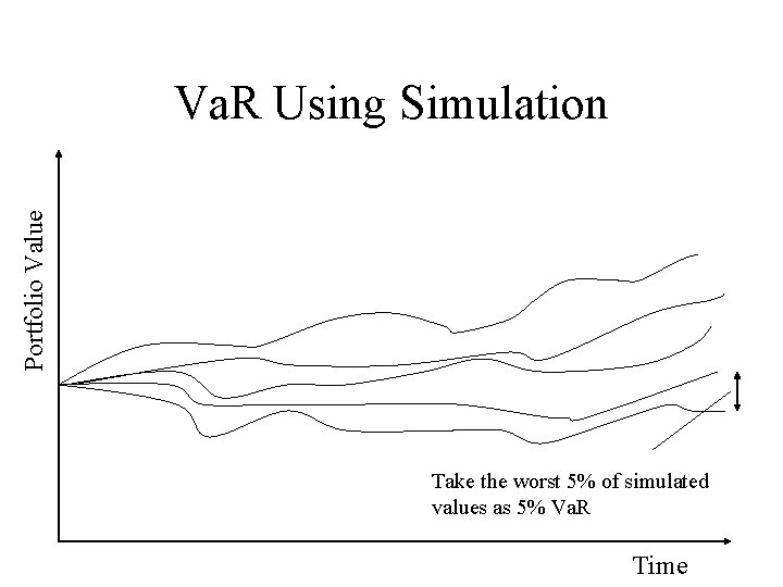
Uses of Simulation • Simulations have many uses and allow us to avoid a lot of complex mathematics • People think you are a rocket scientist if you know about Monte Carlo Simulations • One example would be an alternative approach to calculating the Value-At-Risk • We would generate say 100 future paths for a portfolio’s value by generating a set of 100 simultaneous future paths for each of the assets it contains using either a Monte Carlo or Bootstrap simulation • Out of this 100 we would take the worst 5 or 5% to calculate the 5% Va. R

Portfolio Value Va. R Using Simulation Take the worst 5% of simulated values as 5% Va. R Time

Option Va. R Using Monte Carlo Simulations • One particular use of Monte Carlo simulation is the accurate calculation of Va. R on non-linear portfolios containing options • We generate 100 s of possible paths for the assets on which the options are written and look at the value of the option in each state • We then take the worst 5% or 2. 5% of outcomes to calculate the portfolio 5% or 2. 5% Va. R

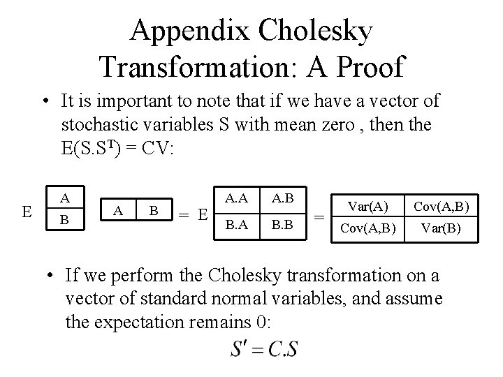
Appendix Cholesky Transformation: A Proof • It is important to note that if we have a vector of stochastic variables S with mean zero , then the E(S. ST) = CV: E A B = E A. A A. B B. A B. B = Var(A) Cov(A, B) Var(B) • If we perform the Cholesky transformation on a vector of standard normal variables, and assume the expectation remains 0:

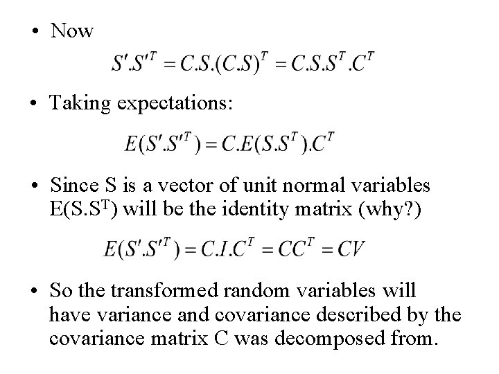
• Now • Taking expectations: • Since S is a vector of unit normal variables E(S. ST) will be the identity matrix (why? ) • So the transformed random variables will have variance and covariance described by the covariance matrix C was decomposed from.