Lecture 1 4 Sampling KotelnikovNyquist Theorem Linear Systems

Lecture 1. 4. Sampling. Kotelnikov-Nyquist Theorem.

Linear Systems Review of Linear Systems • • Linear Time-Invariant Systems Impulse Response Transfer Functions Distortionless Transmission

Linear Time-Invariant Systems • An electronic filter or system is Linear when Superposition holds, that is when, • Where y(t) is the output and x(t) = a 1 x 1(t)+a 2 x 2(t) is the input. • l[. ] denotes the linear (differential equation) system operator acting on [. ]. • If the system is time invariant for any delayed input x(t – t 0), the output is delayed by just the same amount y(t – t 0). • That is, the shape of the response is the same no matter when the input is applied to the system.

Impulse Response x(t)

Impulse Response • The linear time-invariant system without delay blocks is described by a linear ordinary differential equation with constant coefficients and may be characterized by its impulse response h(t). • The impulse response is the solution to the differential equation when the forcing function is a Dirac delta function. y(t) = h(t) when x(t) = δ(t). • In physical networks, the impulse response has to be causal. h(t) = 0 for t < 0 • Generally, an input waveform may be approximated by taking samples of the input at ∆t-second intervals. • Then using the time-invariant and superposition properties, we can obtain the approximate output as • This expression becomes the exact result as ∆t becomes zero. Letting n∆t = λ, we obtain

Transfer Function • The output waveform for a time-invariant network can be obtained by convolving the input waveform with the impulse response of the system. • The impulse response can be used to characterize the response of the system in the time domain. • The spectrum of the output signal is obtained by taking the Fourier transform of both sides. Using the convolution theorem, • Where H(f) = ℑ[h(t)] is transfer function or frequency response of the network. • The impulse response and frequency response are a Fourier transform pair: • Generally, transfer function H(f) is a complex quantity and can be written in polar form.

Transfer Function • The |H(f)| is the Amplitude (or magnitude) Response. • The Phase Response of the network is • Since h(t) is a real function of time (for real networks), it follows 1. |H(f)| is an even function of frequency and 2. θ(f) is an odd function of frequency.

Output for Sinusoidal and periodic Inputs

Power Transfer Function Ø Derive the relationship between the power spectral density (PSD) at the input, Px(f), and that at the output, Py(f) , of a linear time-invariant network. Using the definition of PSD of the output is Using transfer function in a formal sense, we obtain Thus, the power transfer function of the network is

Example 2. 14 RC Low Pass Filter

Example 2. 14 RC Low Pass Filter 3 d. B Point

Distortionless Transmission No Distortion if y(t)=Ax(t-Td) Y(f)=AX(f)e-j 2 f. Td For no distortion at the output of an LTI system, two requirements must be satisfied: 1. The amplitude response is flat. |H(f)| = Constant = A ( No Amplitude Distortion) 2. The phase response is a linear function of frequency. θ(f) = <H(f) = -2πf. Td (No Phase Distortion) Second requirement is often specified equivalently by using the time delay. We define the time delay of the system as: Ø If Td(f) is not constant, there is phase distortion, Because the phase response θ(f), is not a linear function of frequency.

Example 2. 15 Distortion Caused By an RC filter Ø For f <0. 5 f 0, the filter will provide almost distortionless transmission. The error in the magnitude response is less than 0. 5 d. B. The error in the phase is less than 2. 18 (8%). Ø For f <f 0, The error in the magnitude response is less than 3 d. B. The error in the phase is less than 12. 38 (27%). Ø In engineering practice, this type of error is often considered to be tolerable.

Example 2. 15 Distortion Caused By a filter Ø The magnitude response of the RC filter is not constant. Ø Distortion is introduced to the frequencies in the pass band below frequency fo.

Example 2. 15 Distortion Caused By a filter Ø The phase response of the RC filter is not a linear function of frequency. Ø Distortion is introduced to the frequencies in the pass band below frequency fo. Ø The time delay across the RC filter is not constant for all frequencies. Ø Distortion is introduced to the frequencies in the pass band below frequency fo.

Ideal Sampling and Nyquist Theorem Ø Impulse Sampling and Digital Signal Processing (DSP) Ø Ideal Sampling and Reconstruction Ø Nyquist Rate and Aliasing Problem Ø Dimensionality Theorem Ø Reconstruction Using Zero Order Hold.

Bandlimited Waveforms Definition: A waveform w(t) is (Absolutely Bandlimited) to B hertz if W(f) = ℑ [w(t)] = 0 for |f| ≥ B Bandlimited |W(f)| -B 0 B f Definition: A waveform w(t) is (Absolutely Time Limited) if w(t) = 0, for |t| ≥ T Theorem: An absolutely bandlimited waveform cannot be absolutely time limited, and vice versa. A physical waveform that is time limited, may not be absolutely bandlimited, but it may be bandlimited for all practical purposes in the sense that the amplitude spectrum has a negligible level above a certain frequency.

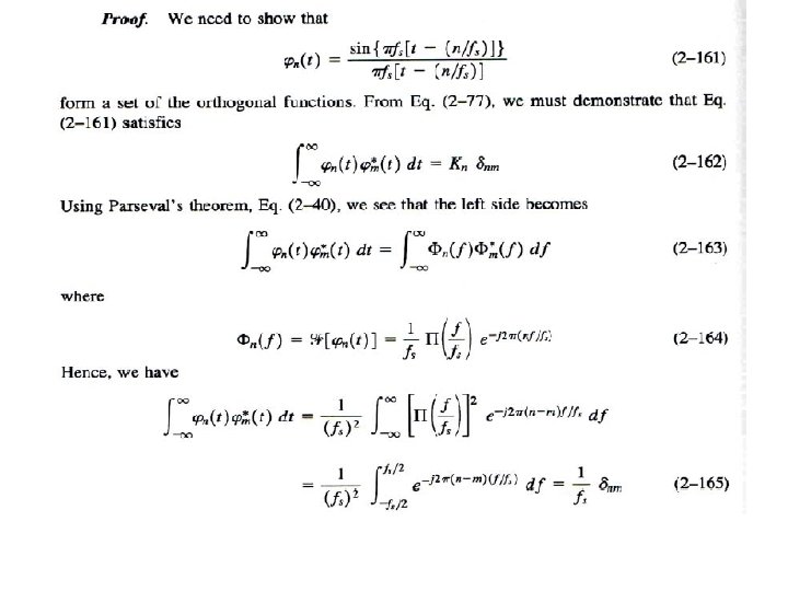
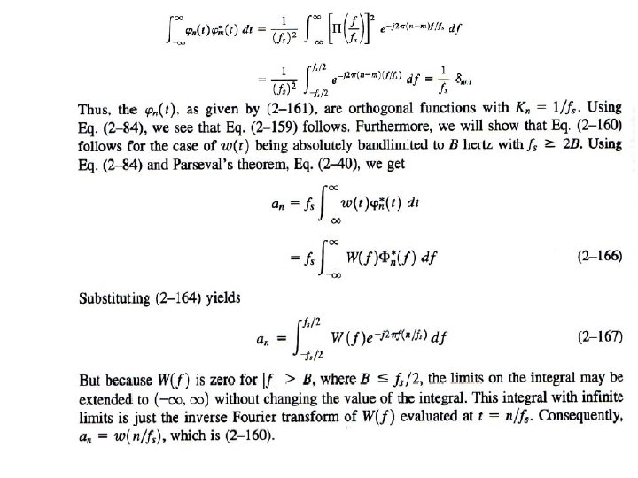
Sampling Theorem: Any physical waveform may be represented over the interval -∞ < t < ∞ by The fs is a parameter called the Sampling Frequency. Furthermore, if w(t) is bandlimited to B Hertz and fs ≥ 2 B, then above expansion becomes the sampling function representation, where an= w(n/fs) That is, for fs ≥ 2 B, the orthogonal series coefficients are simply the values of the waveform that are obtained when the waveform is sampled with a Sampling Period of Ts=1/ fs seconds.

Sampling Theorem Ø The MINIMUM SAMPLING RATE allowed for reconstruction without error is called the NYQUIST FREQUENCY or the Nyquist Rate. Ø Suppose we are interested in reproducing the waveform over a T 0 -sec interval, the minimum number of samples that are needed to reconstruct the waveform is: • There are N orthogonal functions in the reconstruction algorithm. We can say that N is the Number of Dimensions needed to reconstruct the T 0 -second approximation of the waveform. • The sample values may be saved, for example in the memory of a digital computer, so that the waveform may be reconstructed later, or the values may be transmitted over a communication system for waveform reconstruction at the receiving end.

Sampling Theorem

Impulse Sampling and Digital Signal Processing • The impulse-sampled series is another orthogonal series. • It is obtained when the (sin x) / x orthogonal functions of the sampling theorem are replaced by an orthogonal set of delta (impulse) functions. • The impulse-sampled series is identical to the impulse-sampled waveform ws(t): • both can be obtained by multiplying the unsampled waveform by a unit-weight impulse train, yielding Waveform Impulse sampled waveform

Reconstruction of a Sampled Waveform Ø The sampled signal is converted back to a continuous signal by using a reconstruction system such as a low pass filter. x(n. Ts) Ø Same sample values may give different reconstructed signals x 1(t) and x 2(t). Why ? ? ?

Ideal Reconstruction in the Time Domain x(n. Ts) Ø The sampled signal is converted back to a continuous signal by using a reconstruction system such as a low pass filter having a Sa function impulse response Ideal low pass reconstruction filter output. The impulse response of the ideal low pass reconstruction filter.

Spectrum of a Impulse Sampled Waveform The spectrum for the impulse-sampled waveform ws(t) can be evaluated by substituting the Fourier series of the (periodic) impulse train into above Eq. to get By taking the Fourier transform of both sides of this equation, we get

Spectrum of a Impulse Sampled Waveform Ø The spectrum of the impulse sampled signal is the spectrum of the unsampled signal that is repeated every fs Hz, where fs is the sampling frequency (samples/sec). Ø This is quite significant for digital signal processing (DSP). Ø This technique of impulse sampling maybe be used to translate the spectrum of a signal to another frequency band that is centered on some harmonic of the sampling frequency.

Undersampling and Aliasing Ø If fs<2 B, The waveform is Undersampled. The spectrum of ws(t) will consist of overlapped, replicated spectra of w(t). The spectral overlap or tail inversion, is called aliasing or spectral folding. The low-pass filtered version of ws(t) will not be exactly w(t). The recovered w(t) will be distorted because of the aliasing. Low Pass Filter for Reconstruction Notice the distortion on the reconstructed signal due to undersampling

Undersampling and Aliasing Effect of Practical Sampling Notice that the spectral components have decreasing magnitude

Dimensionality Theorem THEOREM: When BT 0 is large, a real waveform may be completely specified by N=2 BT 0 independent pieces of information that will describe the waveform over a T 0 interval. N is said to be the number of dimensions required to specify the waveform, and B is the absolute bandwidth of the waveform. Ø The information which can be conveyed by a bandlimited waveform or a bandlimited communication system is proportional to the product of the bandwidth of that system and the time allowed for transmission of the information. Ø The dimensionality theorem has profound implications in the design and performance of all types of communication systems.

Reconstruction Using a Zero-order Hold Basic System Anti-imaging Filter is used to correct distortions occurring due to non ideal reconstruction

Discrete Processing of Continuous-time Signals Basic System Equivalent Continuous Time System

END