ISy E 6203 Inventory vs Transport John H

ISy. E 6203 Inventory vs Transport John H. Vande Vate Fall 2011 1 1

Dell Projects • Conference call: • 4 -5 PM EST Wednesday 2 2

Agenda • Team Presentations – Financial Statements • Transport & Inventory – How’d you calculate? – What would you do next as VP of SC? • Improving the balance between transport & inventory 3 3

Our Company • Well over $100 million in Cycle Stock at the stores! • How to reduce this? 4 4

First Step • Use full-truck load rates, but don’t fill the trucks • Treat all stores the same • What happens if we ship half a truck load instead of a full truck load? • More generally? If we ship a quantity Q? 5 5

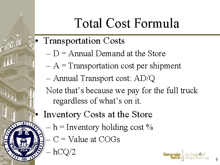
Total Cost Formula • Transportation Costs – D = Annual Demand at the Store – A = Transportation cost per shipment – Annual Transport cost: AD/Q Note that’s because we pay for the full truck regardless of what’s on it. • Inventory Costs at the Store – h = Inventory holding cost % – C = Value at COGs – h. CQ/2 6 6

Total Cost Formula • How does changing the shipment quantity Q affect pipeline inventory? 7 7

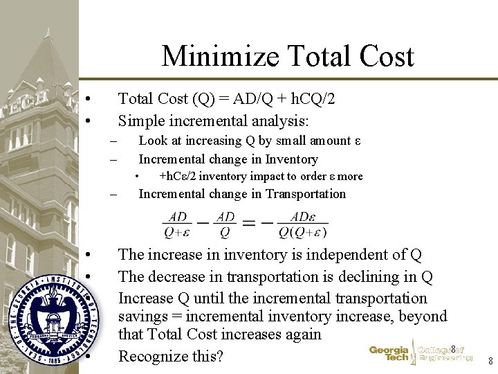
Minimize Total Cost • • Total Cost (Q) = AD/Q + h. CQ/2 Simple incremental analysis: – – Look at increasing Q by small amount ε Incremental change in Inventory • – • • +h. Cε/2 inventory impact to order ε more Incremental change in Transportation The increase in inventory is independent of Q The decrease in transportation is declining in Q Increase Q until the incremental transportation savings = incremental inventory increase, beyond that Total Cost increases again 8 Recognize this? 8

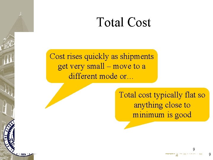
Total Cost rises quickly as shipments get very small – move to a different mode or… Total cost typically flat so anything close to minimum is good 9 9

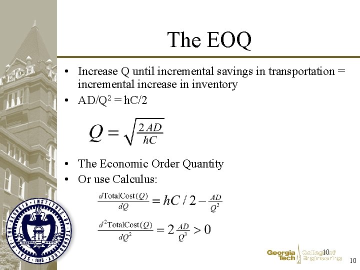
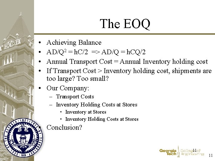
The EOQ • Increase Q until incremental savings in transportation = incremental increase in inventory • AD/Q 2 = h. C/2 • The Economic Order Quantity • Or use Calculus: 10 10

The EOQ • • Achieving Balance AD/Q 2 = h. C/2 => AD/Q = h. CQ/2 Annual Transport Cost = Annual Inventory holding cost If Transport Cost > Inventory holding cost, shipments are too large? Too small? • Our Company: – Transport Costs – Inventory Holding Costs at Stores • Inventory Holding Costs at Stores • Conclusion? 11 11

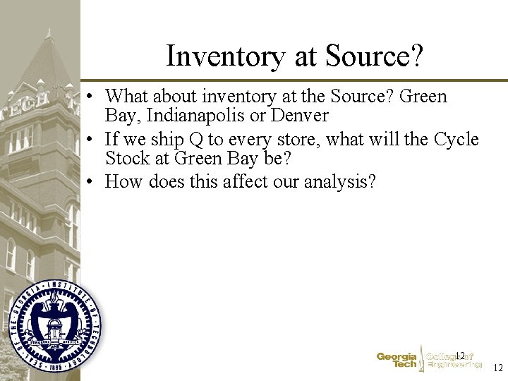
Inventory at Source? • What about inventory at the Source? Green Bay, Indianapolis or Denver • If we ship Q to every store, what will the Cycle Stock at Green Bay be? • How does this affect our analysis? 12 12

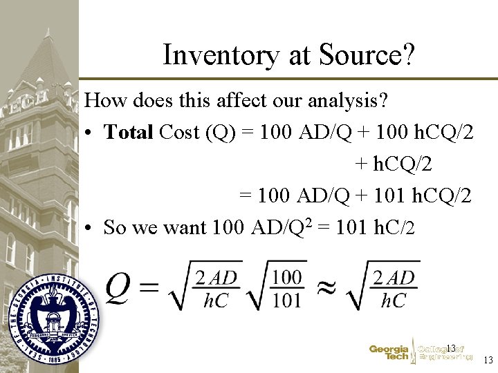
Inventory at Source? How does this affect our analysis? • Total Cost (Q) = 100 AD/Q + 100 h. CQ/2 + h. CQ/2 = 100 AD/Q + 101 h. CQ/2 • So we want 100 AD/Q 2 = 101 h. C/2 13 13

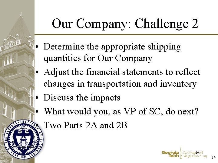
Our Company: Challenge 2 • Determine the appropriate shipping quantities for Our Company • Adjust the financial statements to reflect changes in transportation and inventory • Discuss the impacts • What would you, as VP of SC, do next? • Two Parts 2 A and 2 B 14 14

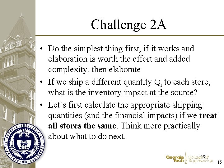
Challenge 2 A • Do the simplest thing first, if it works and elaboration is worth the effort and added complexity, then elaborate • If we ship a different quantity Qi to each store, what is the inventory impact at the source? • Let’s first calculate the appropriate shipping quantities (and the financial impacts) if we treat all stores the same. Think more practically about what to do next. 15 15

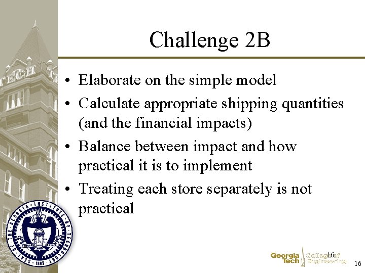
Challenge 2 B • Elaborate on the simple model • Calculate appropriate shipping quantities (and the financial impacts) • Balance between impact and how practical it is to implement • Treating each store separately is not practical 16 16

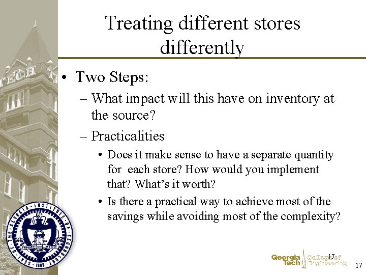
Treating different stores differently • Two Steps: – What impact will this have on inventory at the source? – Practicalities • Does it make sense to have a separate quantity for each store? How would you implement that? What’s it worth? • Is there a practical way to achieve most of the savings while avoiding most of the complexity? 17 17

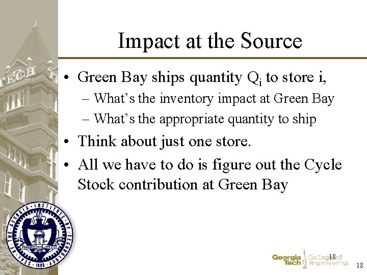
Impact at the Source • Green Bay ships quantity Qi to store i, – What’s the inventory impact at Green Bay – What’s the appropriate quantity to ship • Think about just one store. • All we have to do is figure out the Cycle Stock contribution at Green Bay 18 18

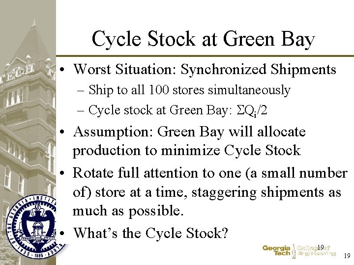
Cycle Stock at Green Bay • Worst Situation: Synchronized Shipments – Ship to all 100 stores simultaneously – Cycle stock at Green Bay: Qi/2 • Assumption: Green Bay will allocate production to minimize Cycle Stock • Rotate full attention to one (a small number of) store at a time, staggering shipments as much as possible. • What’s the Cycle Stock? 19 19

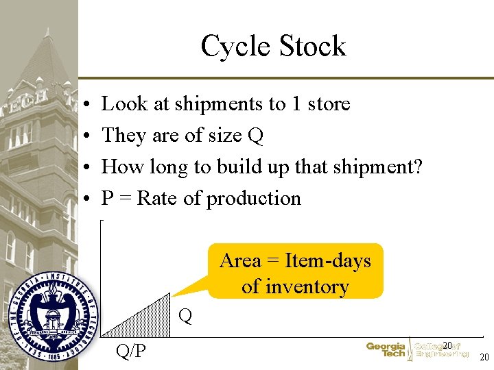
Cycle Stock • • Look at shipments to 1 store They are of size Q How long to build up that shipment? P = Rate of production Area = Item-days of inventory Q Q/P 20 20

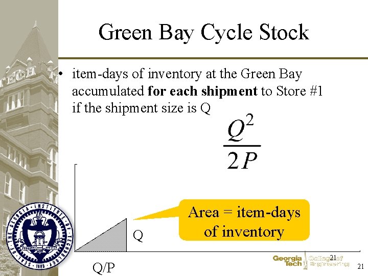
Green Bay Cycle Stock • item-days of inventory at the Green Bay accumulated for each shipment to Store #1 if the shipment size is Q Q Q/P Area = item-days of inventory 21 21

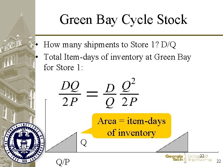
Green Bay Cycle Stock • How many shipments to Store 1? D/Q • Total Item-days of inventory at Green Bay for Store 1: Q Q/P Area = item-days of inventory 22 22

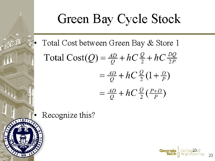
Green Bay Cycle Stock • Total Cost between Green Bay & Store 1 • Recognize this? 23 23

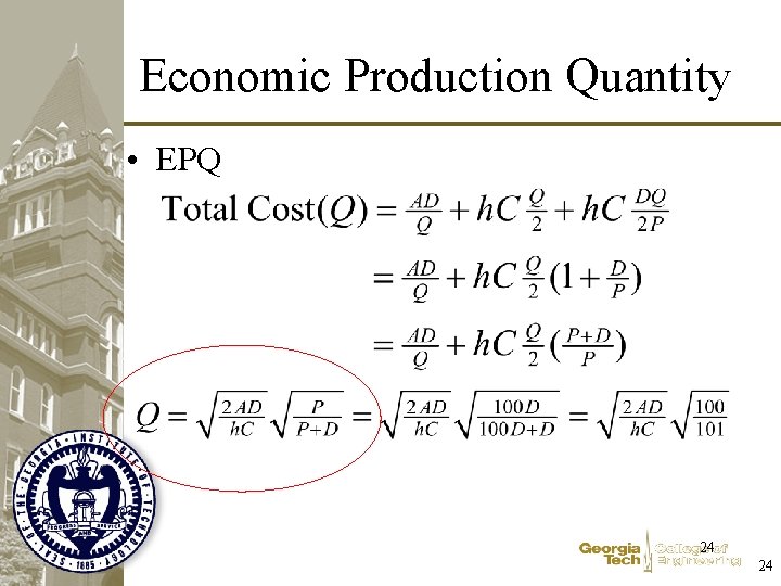
Economic Production Quantity • EPQ 24 24

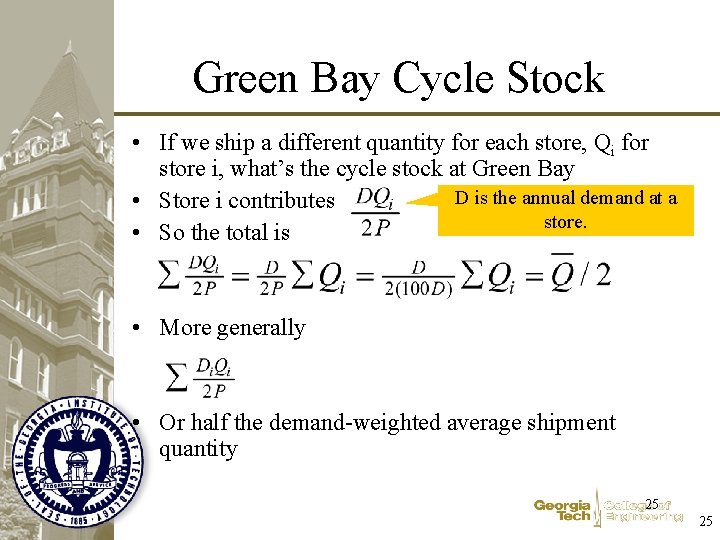
Green Bay Cycle Stock • If we ship a different quantity for each store, Qi for store i, what’s the cycle stock at Green Bay D is the annual demand at a • Store i contributes store. • So the total is • More generally • Or half the demand-weighted average shipment quantity 25 25

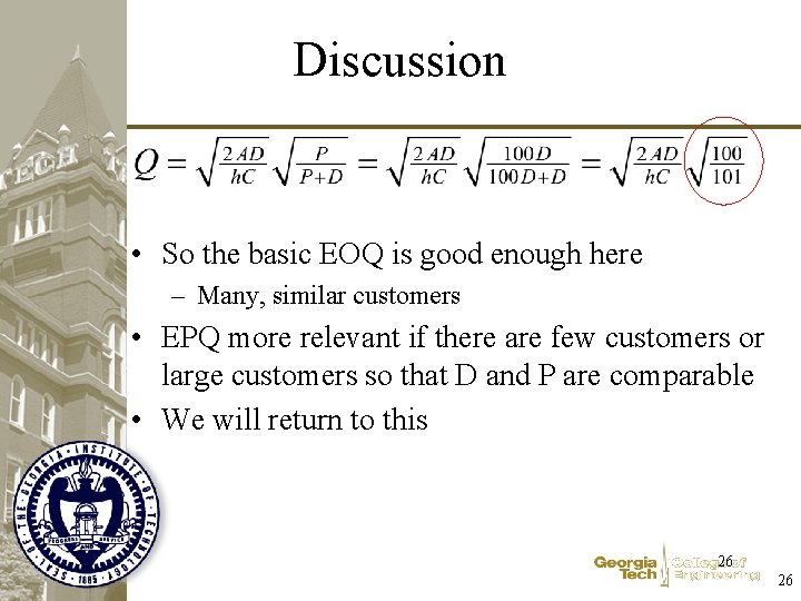
Discussion • So the basic EOQ is good enough here – Many, similar customers • EPQ more relevant if there are few customers or large customers so that D and P are comparable • We will return to this 26 26

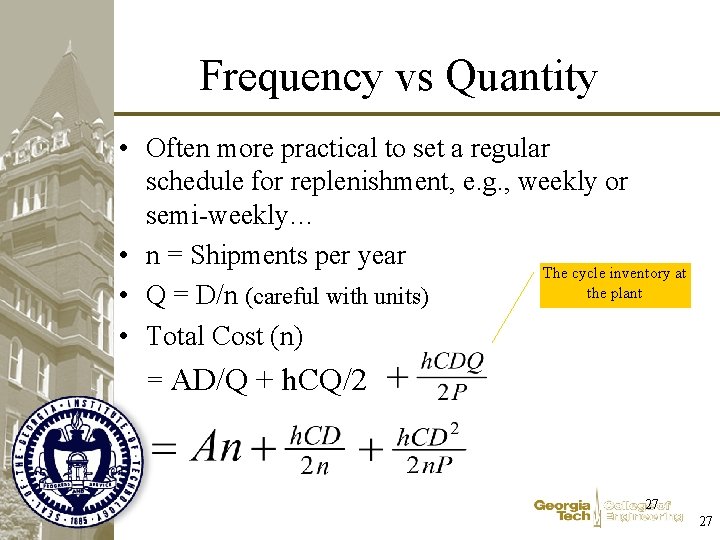
Frequency vs Quantity • Often more practical to set a regular schedule for replenishment, e. g. , weekly or semi-weekly… • n = Shipments per year The cycle inventory at the plant • Q = D/n (careful with units) • Total Cost (n) = AD/Q + h. CQ/2 27 27

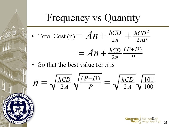
Frequency vs Quantity • Total Cost (n) • So that the best value for n is 28 28

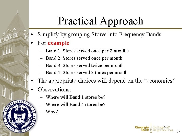
Practical Approach • Simplify by grouping Stores into Frequency Bands • For example: – – Band 1: Stores served once per 2 -months Band 2: Stores served once per month Band 3: Stores served twice per month Band 4: Stores served 3 times per month • The appropriate choices will depend on the “economics” • Observations: – Where will Band 1 stores be? – Where will Band 4 stores be? – Why? 29 29

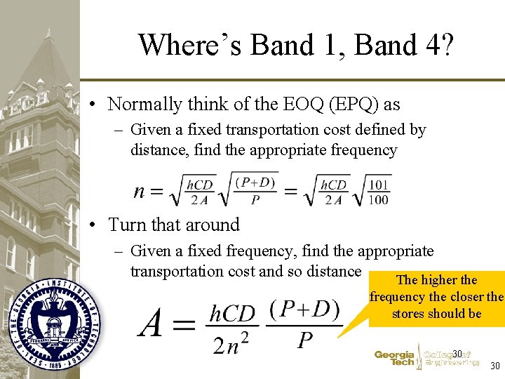
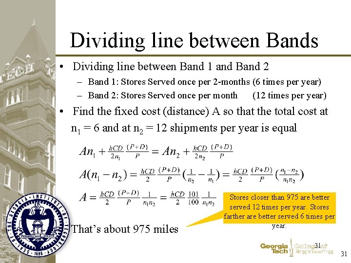
Where’s Band 1, Band 4? • Normally think of the EOQ (EPQ) as – Given a fixed transportation cost defined by distance, find the appropriate frequency • Turn that around – Given a fixed frequency, find the appropriate transportation cost and so distance The higher the frequency the closer the stores should be 30 30

Dividing line between Bands • Dividing line between Band 1 and Band 2 – Band 1: Stores Served once per 2 -months (6 times per year) – Band 2: Stores Served once per month (12 times per year) • Find the fixed cost (distance) A so that the total cost at n 1 = 6 and at n 2 = 12 shipments per year is equal That’s about 975 miles Stores closer than 975 are better served 12 times per year. Stores farther are better served 6 times per year. 31 31

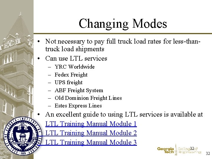
Changing Modes • Not necessary to pay full truck load rates for less-thantruck load shipments • Can use LTL services – – – YRC Worldwide Fedex Freight UPS freight ABF Freight System Old Dominion Freight Lines Estes Express Lines • An excellent guide to using LTL services is available at LTL Training Manual Module 1 LTL Training Manual Module 2 LTL Training Manual Module 3 32 32

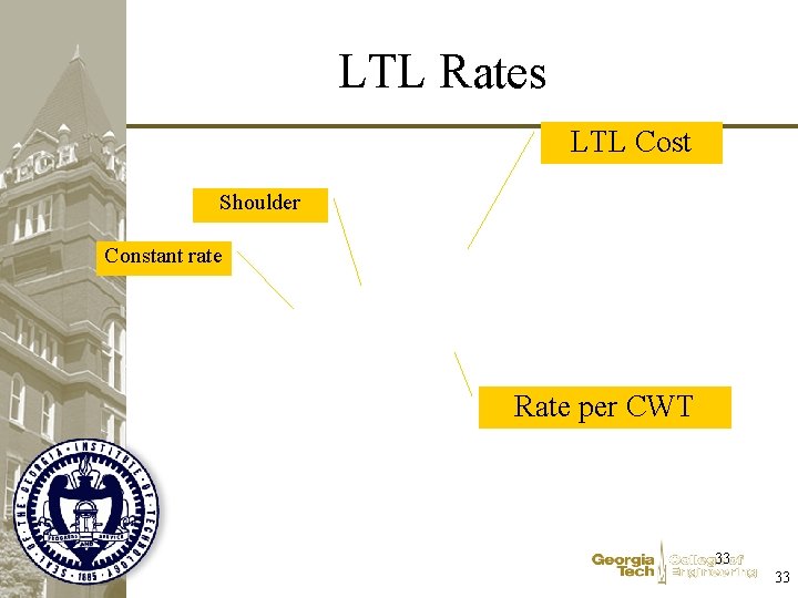
LTL Rates LTL Cost Shoulder Constant rate Rate per CWT 33 33

Observations • Economies of Scale – Although the cost of larger shipments is higher, the rate is lower – This is generally true across modes: Parcel – LTL – Rail Car … • Under LTL we only pay for the portion of the vehicle we use (but at the higher rate) 34 34

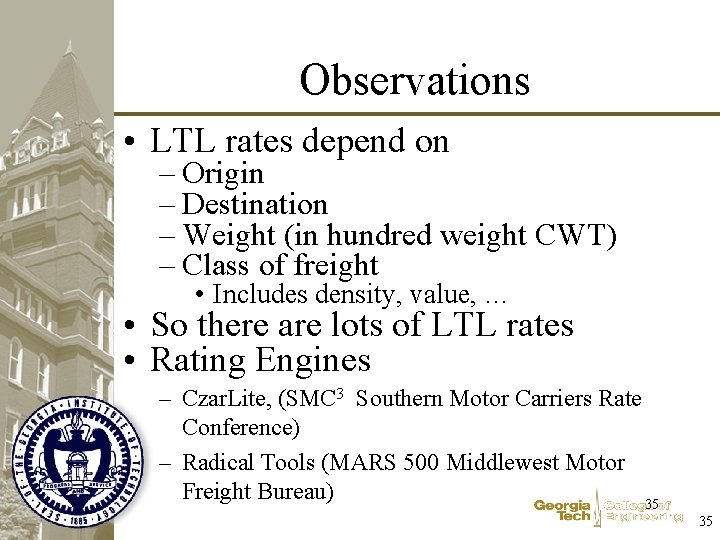
Observations • LTL rates depend on – Origin – Destination – Weight (in hundred weight CWT) – Class of freight • Includes density, value, … • So there are lots of LTL rates • Rating Engines – Czar. Lite, (SMC 3 Southern Motor Carriers Rate Conference) – Radical Tools (MARS 500 Middlewest Motor Freight Bureau) 35 35

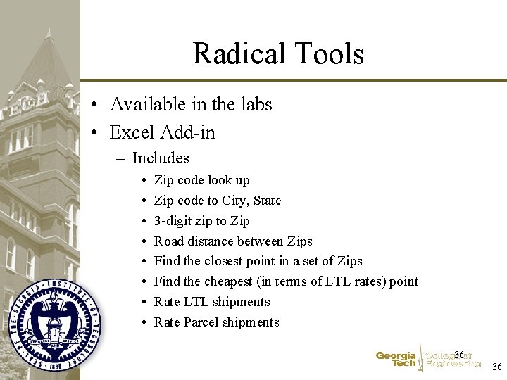
Radical Tools • Available in the labs • Excel Add-in – Includes • • Zip code look up Zip code to City, State 3 -digit zip to Zip Road distance between Zips Find the closest point in a set of Zips Find the cheapest (in terms of LTL rates) point Rate LTL shipments Rate Parcel shipments 36 36

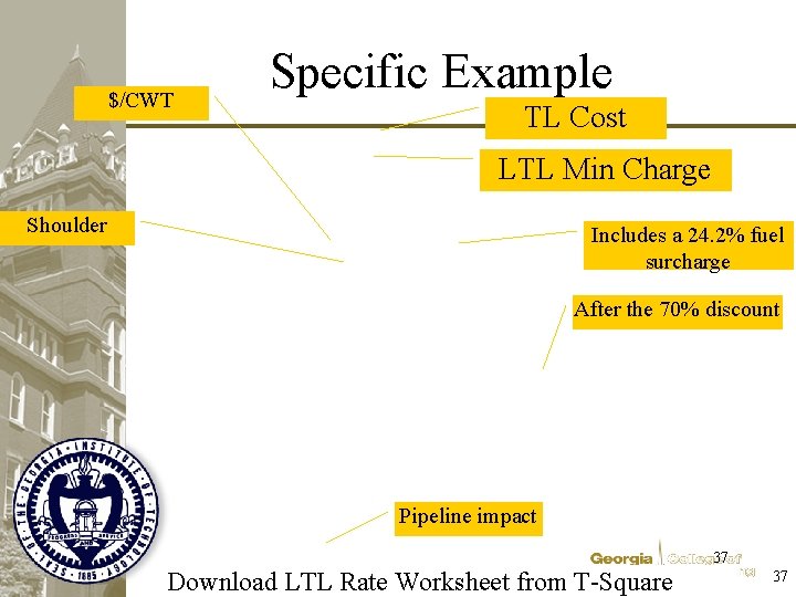
$/CWT Specific Example TL Cost LTL Min Charge Shoulder Includes a 24. 2% fuel surcharge After the 70% discount Pipeline impact 37 Download LTL Rate Worksheet from T-Square 37

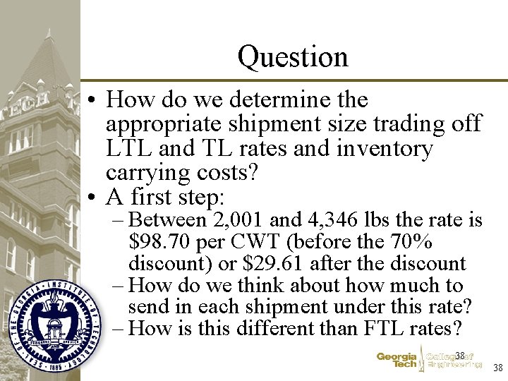
Question • How do we determine the appropriate shipment size trading off LTL and TL rates and inventory carrying costs? • A first step: – Between 2, 001 and 4, 346 lbs the rate is $98. 70 per CWT (before the 70% discount) or $29. 61 after the discount – How do we think about how much to send in each shipment under this rate? – How is this different than FTL rates? 38 38

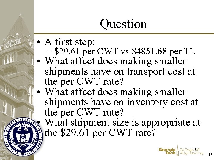
Question • A first step: – $29. 61 per CWT vs $4851. 68 per TL • What affect does making smaller shipments have on transport cost at the per CWT rate? • What affect does making smaller shipments have on inventory cost at the per CWT rate? • What shipment size is appropriate at the $29. 61 per CWT rate? 39 39

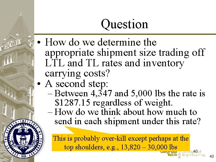
Question • How do we determine the appropriate shipment size trading off LTL and TL rates and inventory carrying costs? • A second step: – Between 4, 347 and 5, 000 lbs the rate is $1287. 15 regardless of weight. – How do we think about how much to send in each shipment under this rate? This is probably over-kill except perhaps at the top shoulders, e. g. , 13, 820 – 30, 000 lbs 40 40

Challenge 3 • Determine the appropriate mode and shipping quantity from Green Bay to Store #2 in Los Angeles. • Briefly describe thinking behind your calculations 41 41

Challenge 4 • Roll this strategy out to all Stores. Determine the appropriate mode and shipping quantity to every store • Remember to keep it practical. • Briefly describe thinking behind your calculations • What are the impacts on SPEED, ROIC and Margin? • What would you do next as VP of SC? 42 42

Warning • Low hanging fruit is mostly picked • We are starting to find it requires more and more work to achieve smaller and smaller impacts • The harder we have to work, the more complex we make the operations – diminishing our impact further • We will have to think smart to be effective • Ideas? 43 43

Economies of Scale in Transport Class 70 LTL rates/lb from Green Bay to LA Shipment weight (lbs) 44 44

Questions? 45 45

The HDT Case • Challenge 5: The HDT Case • Answer the following questions: – Compare the direct costs of the alternatives – Considering cash flow impacts, make a recommendation about which alternative to pursue – Since the buyer pays for the trucks as they are delivered, analyze whether or not it would be advantageous for HDT to pay overtime to speed up production assuming they ship the trucks via Baltimore as soon as they are ready. Assume that HDT’s cost of borrowing is 12% per year. Make reasonable assumptions about the impacts of overtime on production. • Due: ? ? ? 46 46