INTRODUCTORY STATISTICS Chapter 7 The Central Limit Theorem


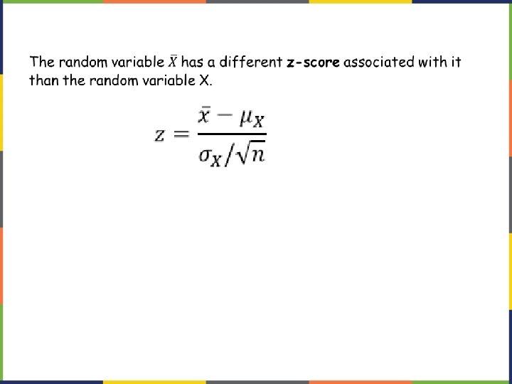
 Suppose X is a random variable with")


 drawn from ANY distribution")


 The print on the package of 100 -watt General Electric soft-white")
 A study involving stress is conducted among the students on a college")
 The annual per capita (average person) chewing gum consumption in the United")
 Based on data from the National Health Survey, women between the ages")
 According to Boeing data, the 757 airliner carries 200 passengers and has")
 Never. Ready batteries has engineered a newer, longer lasting AAA battery. The")
 Your company has a contract to perform preventive maintenance on thousands of")
 A typical adult has an average IQ score of 105 with a")
 Salaries for teachers in a particular elementary school district are normally distributed")
- Slides: 37
INTRODUCTORY STATISTICS Chapter 7 The Central Limit Theorem
CHAPTER 7: THE CENTRAL LIMIT THEOREM 7. 1 The Central Limit Theorem for Sample Means (Averages) 7. 3 Using the Central Limit Theorem
CHAPTER OBJECTIVES By the end of this chapter, the student should be able to: • Recognize central limit theorem problems. • Classify continuous word problems by their distributions. • Apply and interpret the central limit theorem for means.
7. 1 THE CENTRAL LIMIT THEOREM FOR SAMPLE MEANS Introduction Why are we so concerned with means? Two reasons are that they give us a middle ground for comparison and they are easy to calculate. In this chapter, you will study means and the Central Limit Theorem. The Central Limit Theorem (CLT for short) is one of the most powerful and useful ideas in all of statistics. Both alternatives are concerned with drawing finite samples of size n from a population with a known mean, μ, and a known standard deviation, σ.
The first alternative says that if we collect samples of size n and n is "large enough, " calculate each sample's mean, and create a histogram of those means, then the resulting histogram will tend to have an approximate normal bell shape. The second alternative says that if we again collect samples of size n that are "large enough, " calculate the sum of each sample and create a histogram, then the resulting histogram will again tend to have a normal bell-shape. In either case, it does not matter what the distribution of the original population is, or whether you even need to know it. The important fact is that the sample means and the sums tend to follow the normal distribution. For our class, we will focus on the CLT for sample means.
The size of the sample, n, that is required in order to be 'large enough' depends on the original population from which the samples are drawn. If the original population is far from normal then more observations are needed for the sample means or the sample sums to be normal. Sampling is done with replacement.
Collaborative Classroom Activity Part 1: 1. Roll two dice and find the mean of the numbers that you get. 2. Place a dot for each mean value that you obtained on the class dot plot on the white board. 3. Reproduce the dot plot on your paper. 4. Find the mean and the standard deviation of the class means using your calculator.
Part 2: 1. Roll five dice and find the mean of the numbers that you get. Repeat the experiment five times. You should have five means in total. Write them in the table below. Mean 1 Mean 2 Mean 3 Mean 4 Mean 5 2. Place a dot for each mean value that you obtained on the class dot plot on the white board. 3. Reproduce the dot plot on your paper. 4. Find the mean and the standard deviation of the class means using your calculator.
As the number of dice rolled increases from 1 to 2 to 5 to 10, the following is happening: 1. The mean of the sample means remains approximately the same. 2. The spread of the sample means (the standard deviation of the sample means) gets smaller. 3. The graph appears steeper and thinner. You have just demonstrated the Central Limit Theorem (CLT). The Central Limit Theorem tells you that as you increase the number of dice, the sample means tend toward a normal distribution (the sampling distribution).
The Central Limit for Sample Means (Averages) Suppose X is a random variable with a distribution that may be known or unknown (it can be any distribution). Using a subscript that matches the random variable, suppose: a. μx = the mean of X b. σx = the standard deviation of X
The Central Limit Theorem for Sample Means says that if you keep drawing larger and larger samples (like rolling 1, 2, 5, and, finally, 10 dice) and calculating their means, the sample means form their own normal distribution (the sampling distribution). The normal distribution has the same mean as the original distribution and a variance that equals the original variance divided by n, the sample size. n is the number of values that are averaged together not the number of times the experiment is done.
SAMPLING DISTRIBUTION OF THE MEAN The sampling distribution of the mean is formed by taking the mean of samples from a given population The mean of the sample means is equal to the mean of the population from which the samples were drawn. The standard deviation of the distribution is σ divided by the square root of n. (it is called the standard error. )
STANDARD ERROR Standard Deviation for the Distribution of Sample Means What happens to the standard error as the sample size n increases? Experiment with a few numbers in the space on your paper and then write a sentence stating your conclusion.
CENTRAL LIMIT THEOREM
6. The approximation becomes more accurate as n becomes large.
The Central Limit Thereom: For large sample sizes (n >30) drawn from ANY distribution (or for smaller sample sizes, if the original distribution is normally distributed), the sampling distribution of the means has the following properties: 1. The distribution of the sample means is approximately Normal. 2. The mean of the sampling distribution is equal to the mean of the population. 3. The standard deviation of the sampling distribution is equal to the standard deviation of the population divide by the square root of n.
Example 1 An unknown distribution has a mean of 90 and a standard deviation of 15. Samples of size n = 25 are drawn randomly from the population. a. Write the sample distribution in symbolic form. b. Find the probability that the sample mean is between 85 and 92. Draw a graph and shade the area that represents the probability. c. Find the value that is two standard deviations above the expected value, 90, of the sample mean.
Example 2 An unknown distribution has a mean of 45 and a standard deviation of eight. Samples of size n = 30 are drawn randomly from the population. Find the probability that the sample mean is between 42 and 50. Sketch the graph and state all calculator entries.
Example 3 The length of time, in hours, it takes an "over 40" group of people to play one soccer match is normally distributed with a mean of two hours and a standard deviation of 0. 5 hours. A sample of size n = 50 is drawn randomly from the population. Find the probability that the sample mean is between 1. 8 hours and 2. 3 hours.
Example 4 The length of time taken on the SAT for a group of students is normally distributed with a mean of 2. 5 hours and a standard deviation of 0. 25 hours. A sample size of n = 60 is drawn randomly from the population. Find the probability that the sample mean is between two hours and three hours.
Example 5 In a recent study reported Oct. 29, 2012 on the Flurry Blog, the mean age of tablet users is 34 years. Suppose the standard deviation is 15 years. Take a sample of size n = 100. a. What are the mean and standard deviation for the sample mean ages of tablet users? b. What does the distribution look like? c. Find the probability that the sample mean age is more than 30 years (the reported mean age of tablet users in this particular study). d. Find the 95 th percentile for the sample mean age (to one decimal place).
Example 6 In an article on Flurry Blog, a gaming marketing gap for men between the ages of 30 and 40 is identified. You are researching a startup game targeted at the 35 -year-old demographic. Your idea is to develop a strategy game that can be played by men from their late 20 s through their late 30 s. Based on the article’s data, industry research shows that the average strategy player is 28 years old with a standard deviation of 4. 8 years. You take a sample of 100 randomly selected gamers. If your target market is 29 - to 35 -year-olds, should you continue with your development strategy?
Example 7 The mean number of minutes for app engagement by a tablet user is 8. 2 minutes. Suppose the standard deviation is one minute. Take a sample of 60. a. What are the mean and standard deviation for the sample mean number of app engagement by a tablet user? b. What is the standard error of the mean? c. Find the 90 th percentile for the sample mean time for app engagement for a tablet user. Interpret this value in a complete sentence. d. Find the probability that the sample mean is between eight minutes and 8. 5 minutes.
7. 3 USING THE CENTRAL LIMIT THEOREM Using our calculators to find areas under the normal curve, we can use the central limit theorem to make statements as follows: 1. If we take all possible samples of the same (large) size from a population, then about of the sample means will be within one standard deviation of the population mean. 2. If we take one large sample from a population, the probability that this sample mean will be within one standard deviation of the population mean is. This last statement is what we find more useful, since we in real life never look at ALL possible samples, but instead we want to select ONE sample and find the probability that the value of x from this sample falls within a given interval.
Guidelines for applying the CLT • When the original variable is normally distributed, the distribution of the sample means will automatically be normally distributed for any sample size n. • When the distribution of the original variable might not be normal, a sample size of 30 or more is needed to use a normal distribution to approximate the distribution of the sample means. (The larger the sample, the better the approximation will be) Important Note: If you are being asked to find the probability of the mean, use the clt for the mean. If you are being asked to find the probability of an individual value, do not use the clt. Use the distribution of its random variable.
Practice 1. ) The print on the package of 100 -watt General Electric soft-white lightbulbs says that these bulbs have an average life of 750 hours. Assume that the lives of all such bulbs have a normal distribution with a mean of 750 hours and a standard deviation of 55 hours. Find the probability that the mean life of a random sample of 25 such bulbs will be less than 725 hours.
2. ) A study involving stress is conducted among the students on a college campus. The stress scores follow a uniform distribution with the lowest stress score equal to one and the highest equal to five. Using a sample of 75 students, find: a. ) The probability that the mean stress score for the 75 students is less than two. b. ) The 90 th percentile for the mean stress score for the 75 students.
3. ) The annual per capita (average person) chewing gum consumption in the United States is 200 pieces. Suppose that the standard deviation of per capita consumption of chewing gum is 145 pieces per year. a) Find the probability that the average annual chewing gum consumption of 84 randomly selected Americans is more than 220 pieces. b) Find the probability that the average annual chewing gum consumption of 84 randomly selected Americans is within 100 pieces of the population mean. c) Find the probability that the average annual chewing gum consumption of 16 randomly selected Americans is less than 100 pieces.
4. ) Based on data from the National Health Survey, women between the ages of 18 and 24 have an average systolic blood pressures (in mm Hg) of 114. 8 with a standard deviation of 13. 1. Systolic blood pressure for women between the ages of 18 to 24 follow a normal distribution. a. If one woman from this population is randomly selected, find the probability that her systolic blood pressure is greater than 120. b. If 40 women from this population are randomly selected, find the probability that their mean systolic blood pressure is greater than 120. c. If the sample were four women between the ages of 18 to 24 and we did not know the original distribution, could the central limit theorem be used?
5. ) According to Boeing data, the 757 airliner carries 200 passengers and has doors with a mean height of 72 inches. Assume for a certain population of men we have a mean of 69. 0 inches and a standard deviation of 2. 8 inches. a. What mean doorway height would allow 95% of men to enter the aircraft without bending? b. Assume that half of the 200 passengers are men. What mean doorway height satisfies the condition that there is a 0. 95 probability that this height is greater than the mean height of 100 men? c. For engineers designing the 757, which result is more relevant: the height from part a or part b? Why?
6. ) Never. Ready batteries has engineered a newer, longer lasting AAA battery. The company claims this battery has an average life span of 17 hours with a standard deviation of 0. 8 hours. Your statistics class questions this claim. As a class, you randomly select 30 batteries and find that the sample mean life span is 16. 7 hours. If the process is working properly, what is the probability of getting a random sample of 30 batteries in which the sample mean lifetime is 16. 7 hours or less? Is the company’s claim reasonable?
7. ) Your company has a contract to perform preventive maintenance on thousands of air-conditioners in a large city. Based on service records from previous years, the time that a technician spends servicing a unit averages one hour with a standard deviation of one hour. In the coming week, your company will service a simple random sample of 70 units in the city. You plan to budget an average of 1. 1 hours per technician to complete the work. Will this be enough time?
8. ) A typical adult has an average IQ score of 105 with a standard deviation of 20. If 20 randomly selected adults are given an IQ test, what is the probability that the sample mean scores will be between 85 and 125 points?
9. ) Salaries for teachers in a particular elementary school district are normally distributed with a mean of $44, 000 and a standard deviation of $6, 500. We randomly survey ten teachers from that district. a. Find the 90 th percentile for an individual teacher’s salary. b. Find the 90 th percentile for the average teacher’s salary.