Central limit theorem outlines Central limit theorem CLT

Central limit theorem ( outlines) : Central limit theorem CLT Hypothesis testing Correction for a finite population Assessing the normality

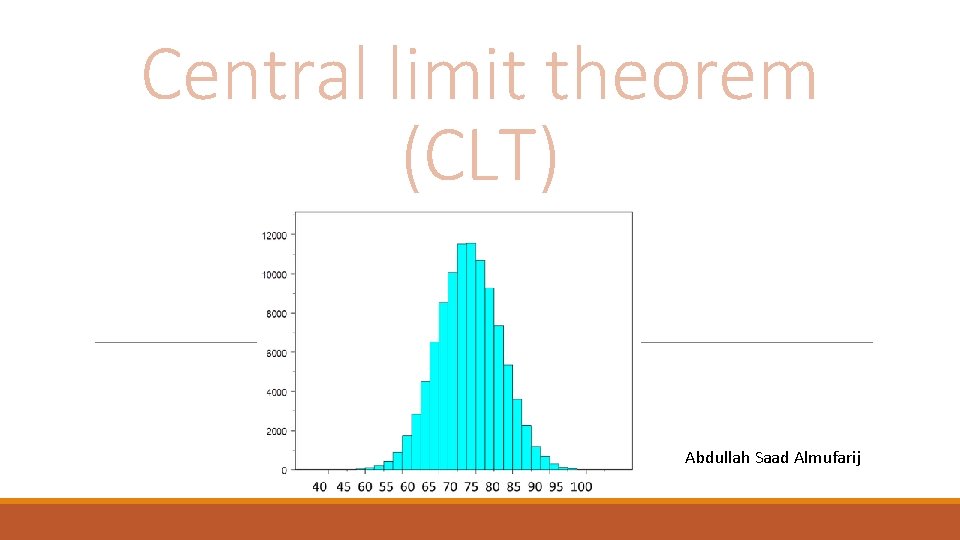
Central limit theorem (CLT) Abdullah Saad Almufarij

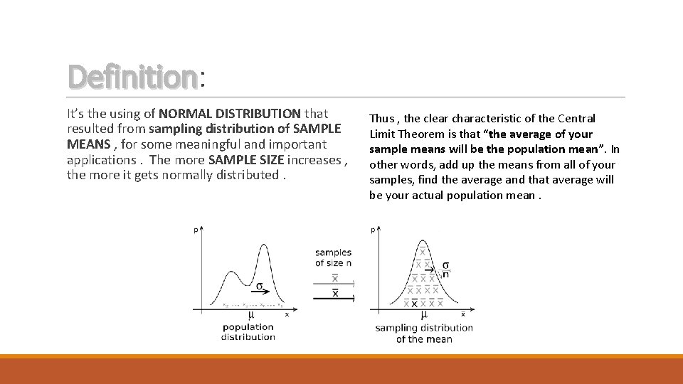
Definition: Definition It’s the using of NORMAL DISTRIBUTION that resulted from sampling distribution of SAMPLE MEANS , for some meaningful and important applications. The more SAMPLE SIZE increases , the more it gets normally distributed. Thus , the clear characteristic of the Central Limit Theorem is that “the average of your sample means will be the population mean”. In other words, add up the means from all of your samples, find the average and that average will be your actual population mean.

Simply : Sampling distribution of the mean Typically, you perform a study for one time , and you might calculate the mean of that one sample. Then , you repeat the study many times and collect the sample size for each one. The next step is you calculate the mean for each of these samples and graph them on a histogram. The histogram displays the distribution of sample means, which statisticians refer to as the sampling distribution of the mean and that is the CENTRAL LIMIT THEOREM (CLT).

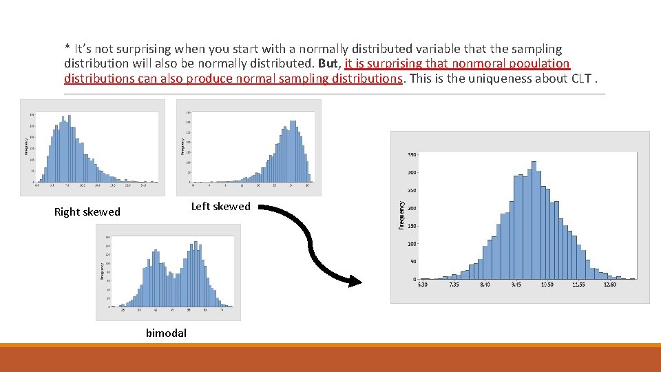
* It’s not surprising when you start with a normally distributed variable that the sampling distribution will also be normally distributed. But, it is surprising that nonmoral population distributions can also produce normal sampling distributions. This is the uniqueness about CLT. Left skewed Right skewed bimodal

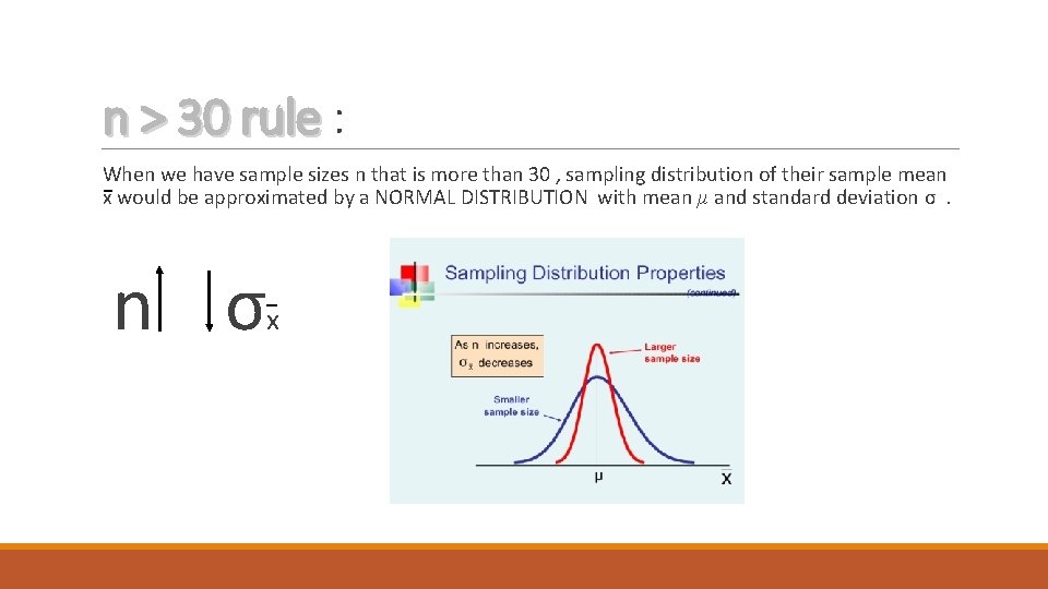
n > 30 rule : When we have sample sizes n that is more than 30 , sampling distribution of their sample mean x would be approximated by a NORMAL DISTRIBUTION with mean μ and standard deviation σ. n σ x

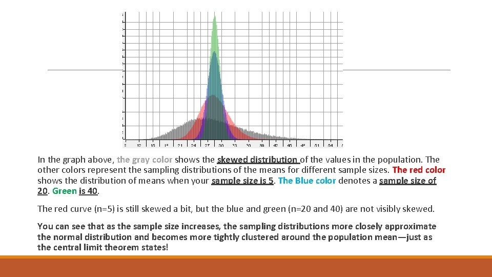
In the graph above, the gray color shows the skewed distribution of the values in the population. The other colors represent the sampling distributions of the means for different sample sizes. The red color shows the distribution of means when your sample size is 5. The Blue color denotes a sample size of 20. Green is 40. The red curve (n=5) is still skewed a bit, but the blue and green (n=20 and 40) are not visibly skewed. You can see that as the sample size increases, the sampling distributions more closely approximate the normal distribution and becomes more tightly clustered around the population mean—just as the central limit theorem states!

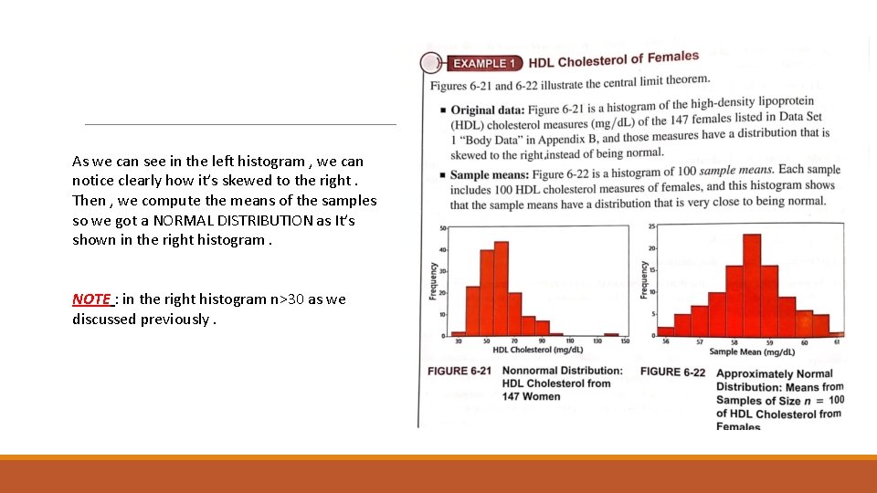
As we can see in the left histogram , we can notice clearly how it’s skewed to the right. Then , we compute the means of the samples so we got a NORMAL DISTRIBUTION as It’s shown in the right histogram. NOTE : in the right histogram n>30 as we discussed previously.

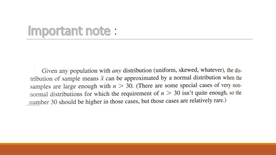
Important note :

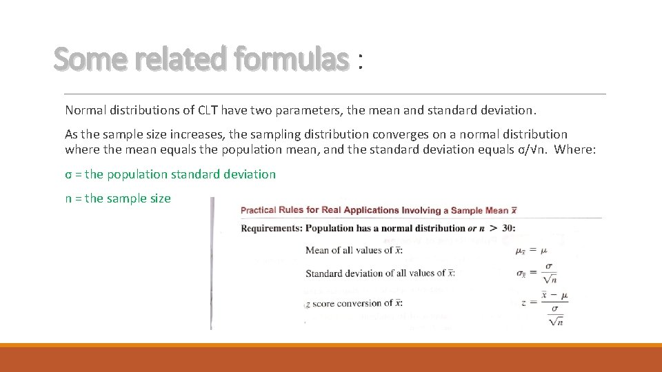
Some related formulas : Normal distributions of CLT have two parameters, the mean and standard deviation. As the sample size increases, the sampling distribution converges on a normal distribution where the mean equals the population mean, and the standard deviation equals σ/√n. Where: σ = the population standard deviation n = the sample size

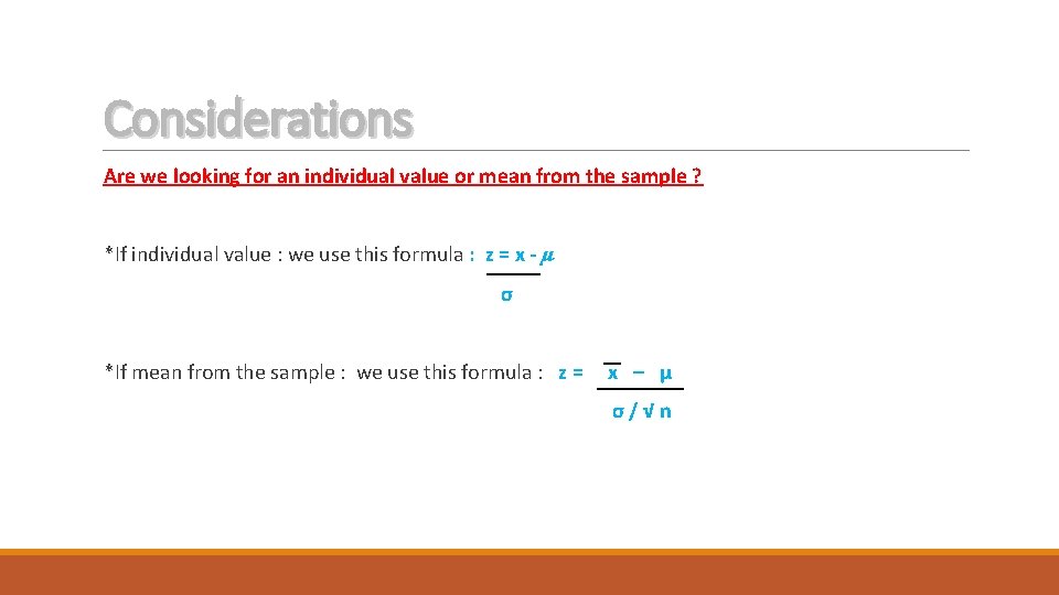
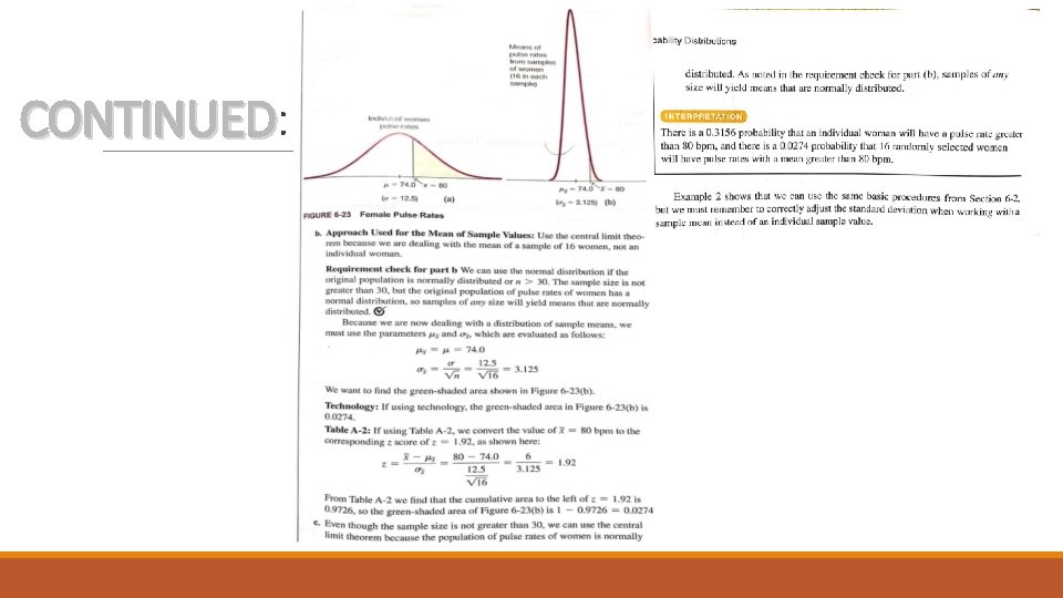
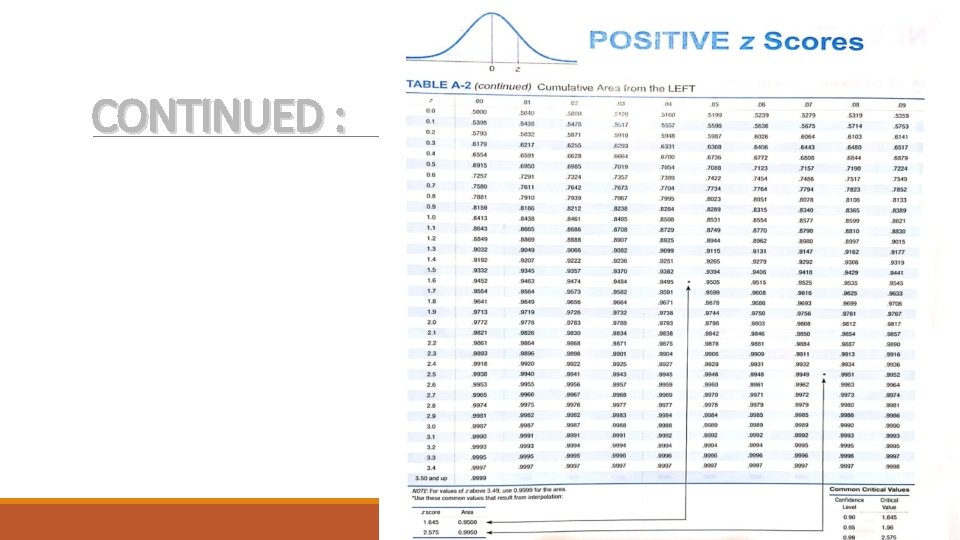
Considerations Are we looking for an individual value or mean from the sample ? *If individual value : we use this formula : z = x - μ σ *If mean from the sample : we use this formula : z = x – μ σ/√n

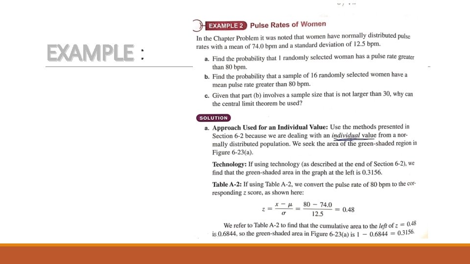
EXAMPLE :

CONTINUED: CONTINUED

CONTINUED :

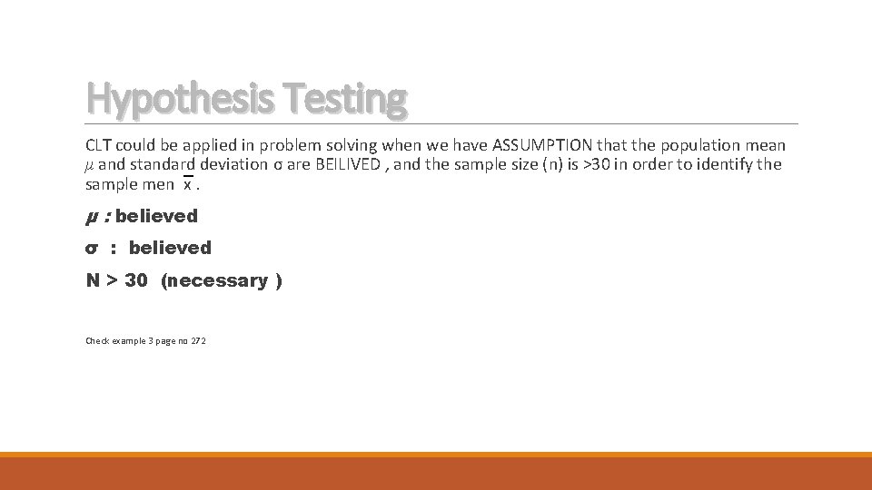
Hypothesis Testing CLT could be applied in problem solving when we have ASSUMPTION that the population mean μ and standard deviation σ are BEILIVED , and the sample size (n) is >30 in order to identify the sample men x. μ : believed σ : believed N > 30 (necessary ) Check example 3 page no 272

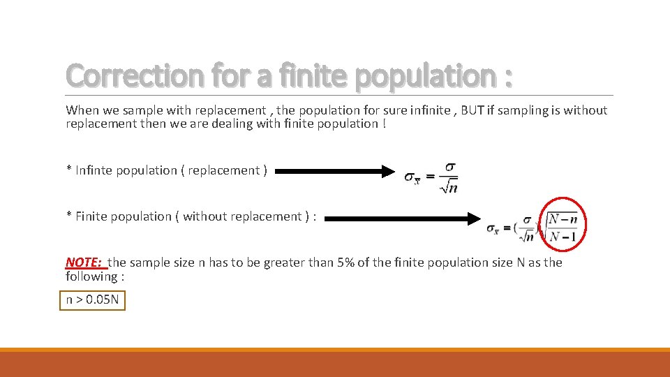
Correction for a finite population : When we sample with replacement , the population for sure infinite , BUT if sampling is without replacement then we are dealing with finite population ! * Infinte population ( replacement ) * Finite population ( without replacement ) : NOTE: the sample size n has to be greater than 5% of the finite population size N as the following : n > 0. 05 N

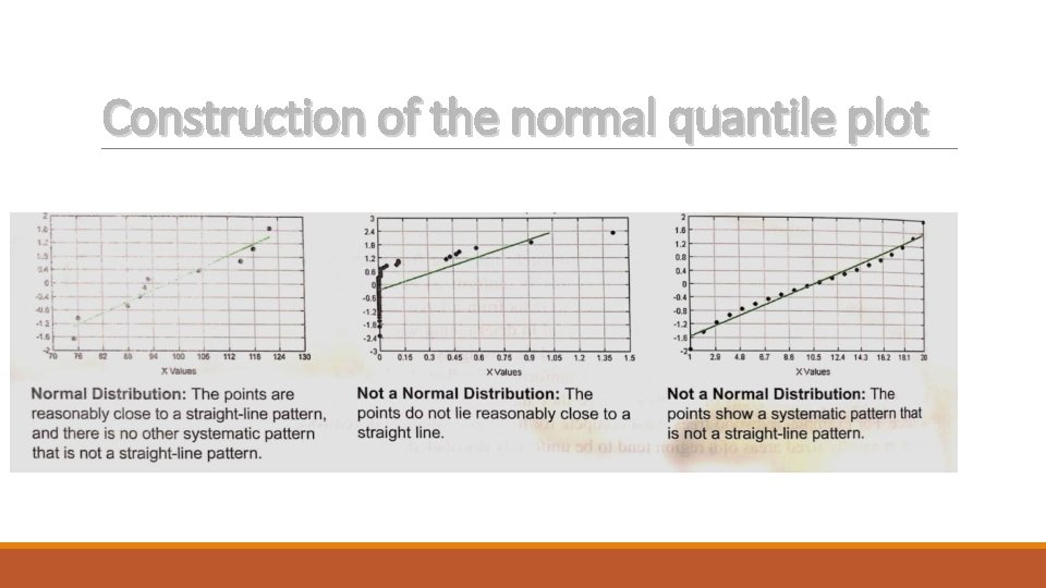
Assessing normality : The criteria to assess normality of a distribution are the followings : 1 - Visual inspection of the histogram 2 - Identification of any outliers 3 - constructing the normal quantile plot

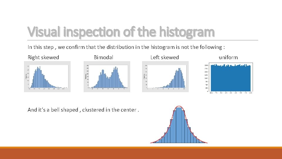
Visual inspection of the histogram In this step , we confirm that the distribution in the histogram is not the following : Right skewed Bimodal And it’s a bell shaped , clustered in the center. Left skewed uniform

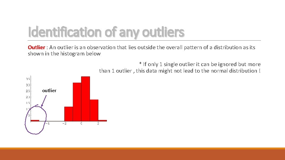
Identification of any outliers Outlier : An outlier is an observation that lies outside the overall pattern of a distribution as its shown in the histogram below * If only 1 single outlier it can be ignored but more than 1 outlier , this data might not lead to the normal distribution ! outlier

Construction of the normal quantile plot

Normal as Approximation to Binomial Distribution Abdulrahman Alzoman

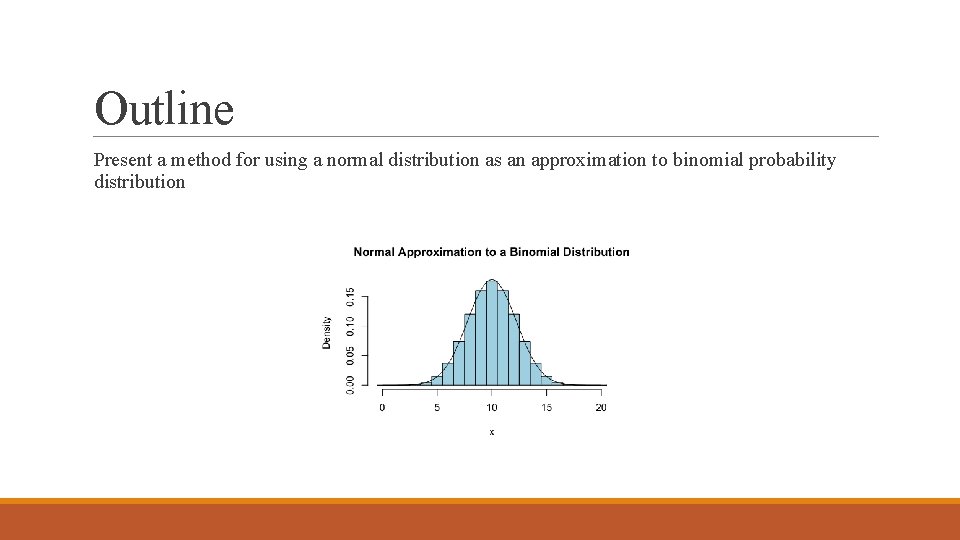
Outline Present a method for using a normal distribution as an approximation to binomial probability distribution

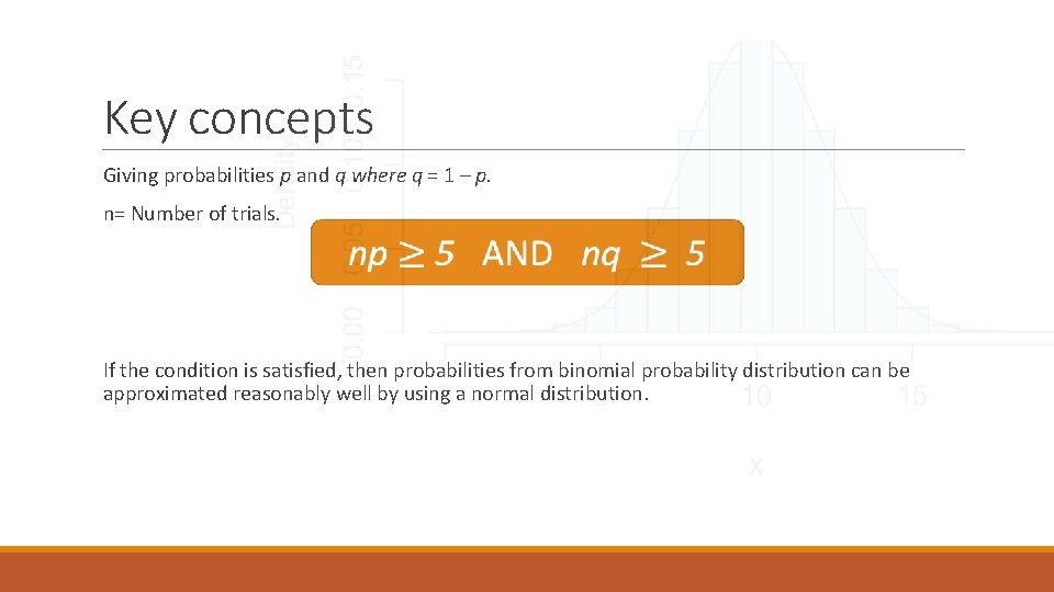
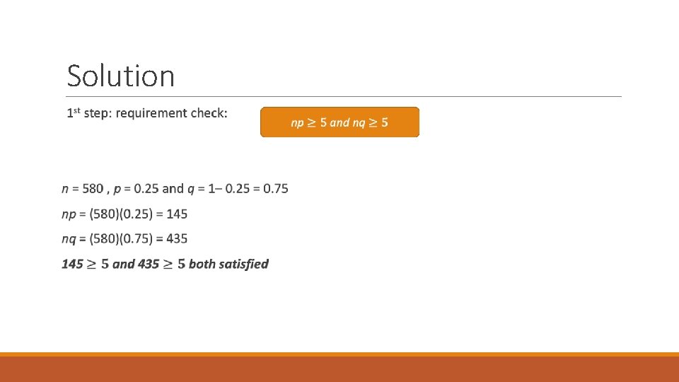
Key concepts Giving probabilities p and q where q = 1 – p. n= Number of trials. If the condition is satisfied, then probabilities from binomial probability distribution can be approximated reasonably well by using a normal distribution.

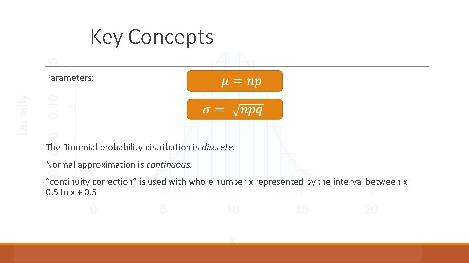
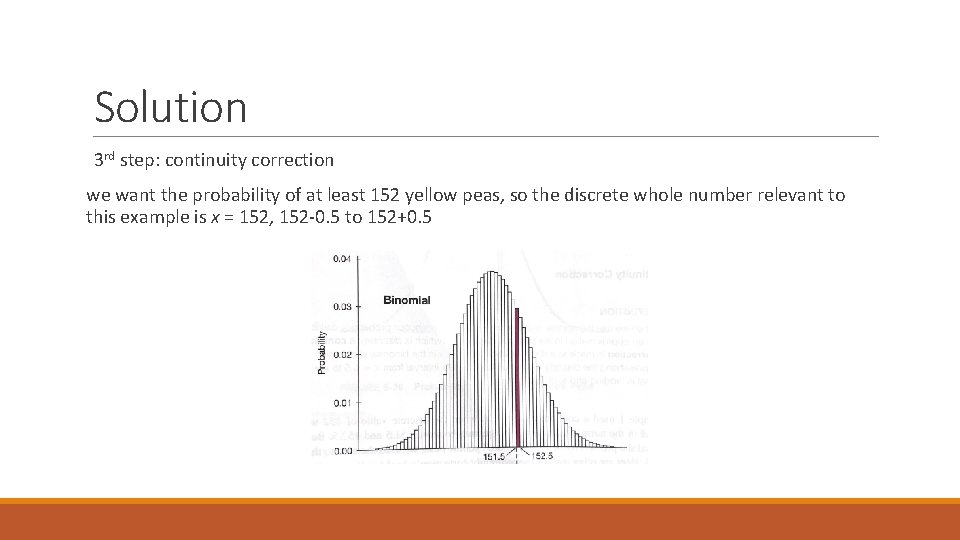
Key Concepts Parameters: The Binomial probability distribution is discrete. Normal approximation is continuous. “continuity correction” is used with whole number x represented by the interval between x – 0. 5 to x + 0. 5

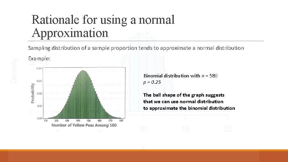
Rationale for using a normal Approximation Sampling distribution of a sample proportion tends to approximate a normal distribution Example: Binomial distribution with n = 580 p = 0. 25 The ball shape of the graph suggests that we can use normal distribution to approximate the binomial distribution

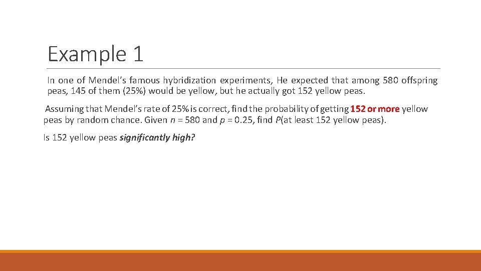
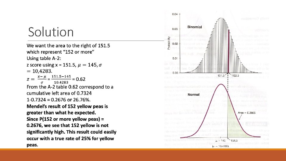
Example 1 In one of Mendel’s famous hybridization experiments, He expected that among 580 offspring peas, 145 of them (25%) would be yellow, but he actually got 152 yellow peas. Assuming that Mendel’s rate of 25% is correct, find the probability of getting 152 or more yellow peas by random chance. Given n = 580 and p = 0. 25, find P(at least 152 yellow peas). Is 152 yellow peas significantly high?

Solution

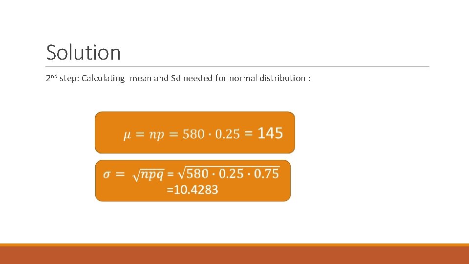
Solution 2 nd step: Calculating mean and Sd needed for normal distribution :

Solution 3 rd step: continuity correction we want the probability of at least 152 yellow peas, so the discrete whole number relevant to this example is x = 152, 152 -0. 5 to 152+0. 5

Solution

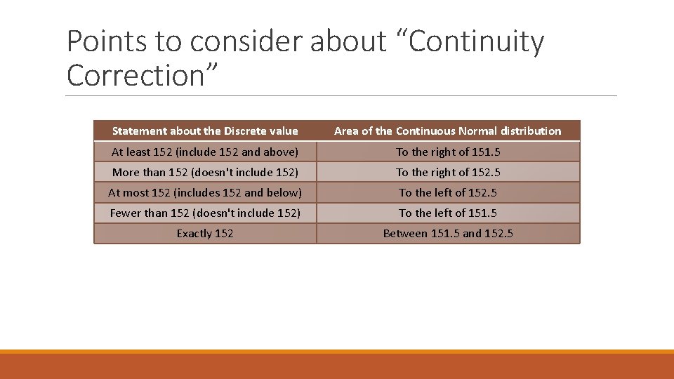
Points to consider about “Continuity Correction” In the previous example we used continuity correction when the discrete value of 152 was represented in the normal distribution by the area between 151. 5 to 152. 5. Because we wanted the probability of “ 152 or more” yellow peas, we used the area to the right of 151. 5

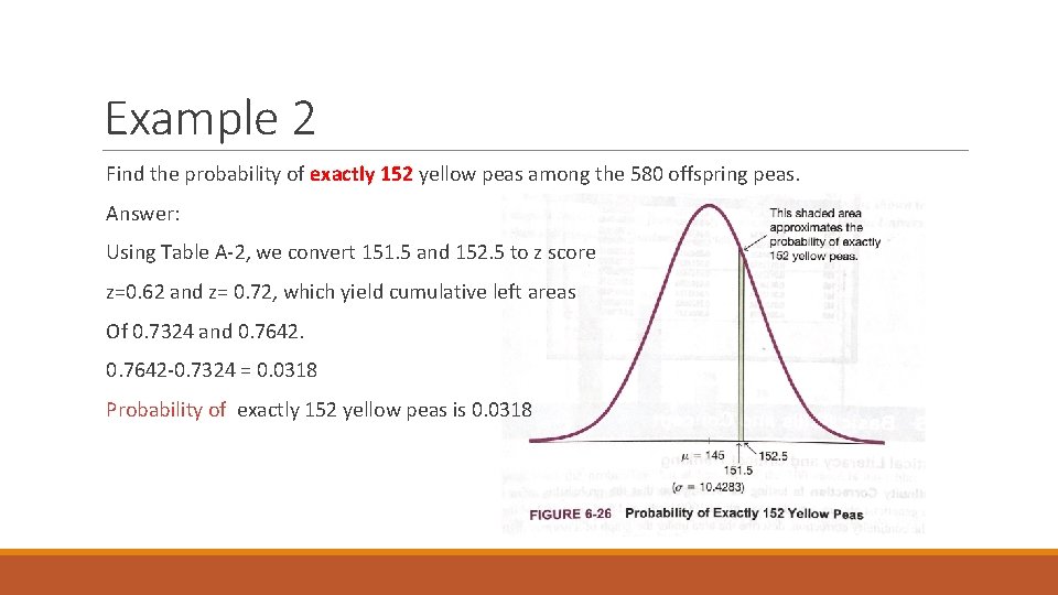
Points to consider about “Continuity Correction” Statement about the Discrete value Area of the Continuous Normal distribution At least 152 (include 152 and above) To the right of 151. 5 More than 152 (doesn't include 152) To the right of 152. 5 At most 152 (includes 152 and below) To the left of 152. 5 Fewer than 152 (doesn't include 152) To the left of 151. 5 Exactly 152 Between 151. 5 and 152. 5

Example 2 Find the probability of exactly 152 yellow peas among the 580 offspring peas. Answer: Using Table A-2, we convert 151. 5 and 152. 5 to z score z=0. 62 and z= 0. 72, which yield cumulative left areas Of 0. 7324 and 0. 7642 -0. 7324 = 0. 0318 Probability of exactly 152 yellow peas is 0. 0318

We saw that x successes among n trials is significantly high if the probability of x or more successes is unlikely with a probability of 0. 05 or less. For this example we should consider the probability of 152 or more yellow peas not exactly 152 as the result of 0. 0318 is not relevant probability.

Thank You! Questions?