The Central Limit Theorem Honors Statistics Lesson 7
- Slides: 33

The Central Limit Theorem Honors Statistics Lesson 7. 4

Objectives/Assignment • How to find sampling distributions and verify their properties • How to interpret the Central Limit Theorem • How to apply the Central Limit Theorem to find the probability of a sample mean

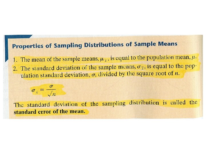
Introduction • In previous sections, you studied the relationship between the mean of a population and values of random variable. In this section, you will study the relationship between a population mean and the means of samples taken from the population. • Definition: A sampling distribution is the probability distribution of a sample statistic that is formed when samples of sizes n are repeatedly taken from a population. If the sample statistic is the sample mean, then the distribution is the sampling distribution of sample means.

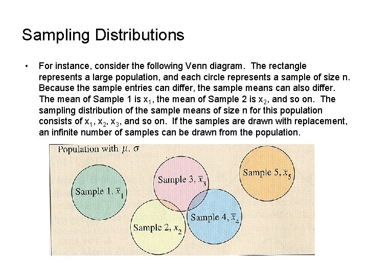
Sampling Distributions • For instance, consider the following Venn diagram. The rectangle represents a large population, and each circle represents a sample of size n. Because the sample entries can differ, the sample means can also differ. The mean of Sample 1 is x 1, the mean of Sample 2 is x 2, and so on. The sampling distribution of the sample means of size n for this population consists of x 1, x 2, x 3, and so on. If the samples are drawn with replacement, an infinite number of samples can be drawn from the population.


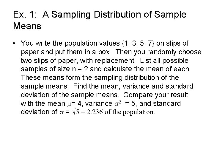
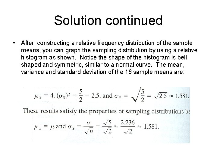
Ex. 1: A Sampling Distribution of Sample Means • You write the population values {1, 3, 5, 7} on slips of paper and put them in a box. Then you randomly choose two slips of paper, with replacement. List all possible samples of size n = 2 and calculate the mean of each. These means form the sampling distribution of the sample means. Find the mean, variance and standard deviation of the sample means. Compare your result with the mean = 4, variance 2 = 5, and standard deviation of = √ 5 = 2. 236 of the population.

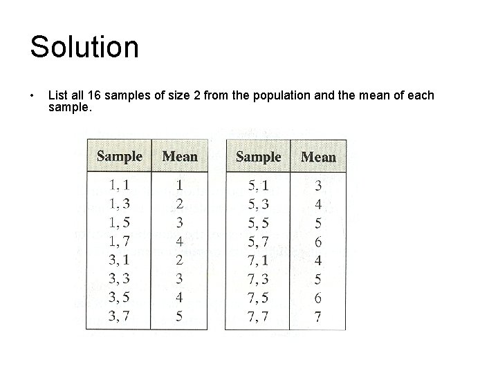
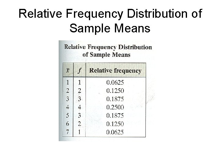
Solution • List all 16 samples of size 2 from the population and the mean of each sample.

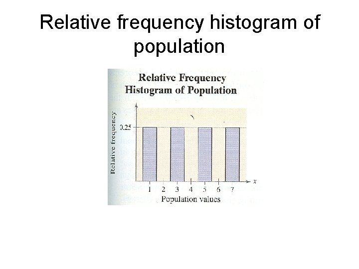
Relative frequency histogram of population

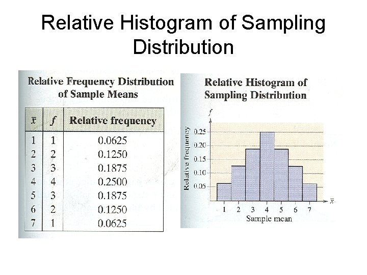
Relative Frequency Distribution of Sample Means

Relative Histogram of Sampling Distribution

Solution continued • After constructing a relative frequency distribution of the sample means, you can graph the sampling distribution by using a relative histogram as shown. Notice the shape of the histogram is bell shaped and symmetric, similar to a normal curve. The mean, variance and standard deviation of the 16 sample means are:

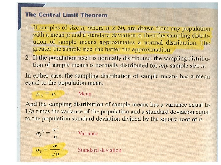
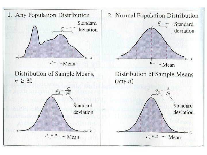
The Central Limit Theorem • The Central Limit Theorem is one of the most important and useful theorems in statistics. This theorem forms the foundation for the inferential branch of statistics. The Central Limit Theorem describes the relationship between the sampling distribution of sample means and the population that the samples are taken from.


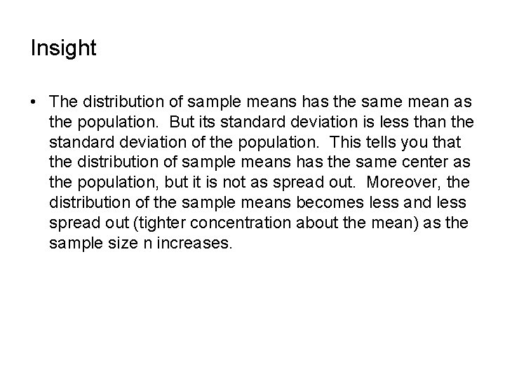
Insight • The distribution of sample means has the same mean as the population. But its standard deviation is less than the standard deviation of the population. This tells you that the distribution of sample means has the same center as the population, but it is not as spread out. Moreover, the distribution of the sample means becomes less and less spread out (tighter concentration about the mean) as the sample size n increases.


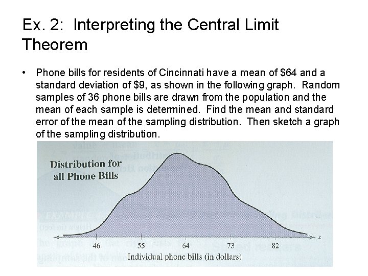
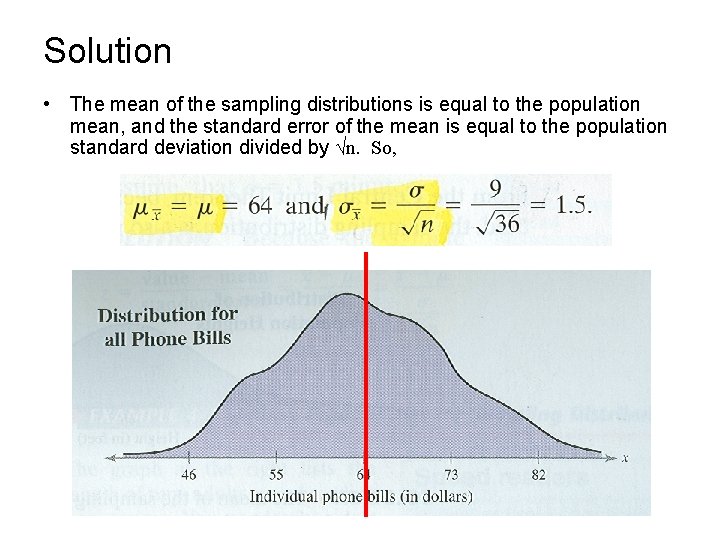
Ex. 2: Interpreting the Central Limit Theorem • Phone bills for residents of Cincinnati have a mean of $64 and a standard deviation of $9, as shown in the following graph. Random samples of 36 phone bills are drawn from the population and the mean of each sample is determined. Find the mean and standard error of the mean of the sampling distribution. Then sketch a graph of the sampling distribution.

Solution • The mean of the sampling distributions is equal to the population mean, and the standard error of the mean is equal to the population standard deviation divided by √n. So,

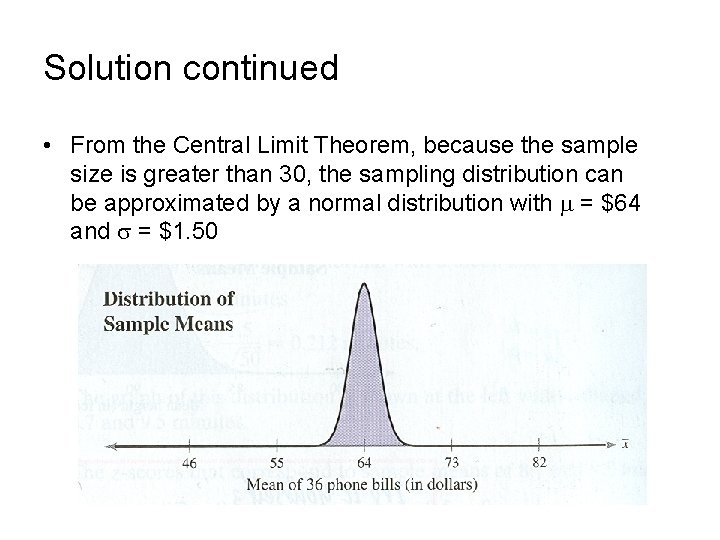
Solution continued • From the Central Limit Theorem, because the sample size is greater than 30, the sampling distribution can be approximated by a normal distribution with = $64 and = $1. 50

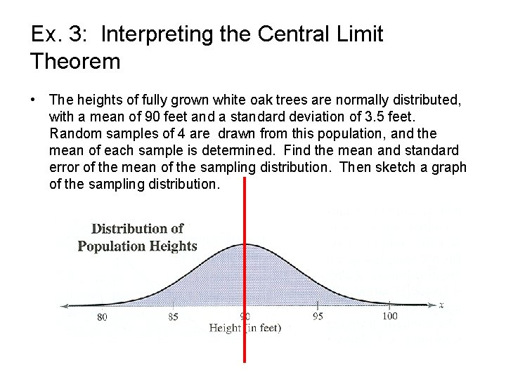
Ex. 3: Interpreting the Central Limit Theorem • The heights of fully grown white oak trees are normally distributed, with a mean of 90 feet and a standard deviation of 3. 5 feet. Random samples of 4 are drawn from this population, and the mean of each sample is determined. Find the mean and standard error of the mean of the sampling distribution. Then sketch a graph of the sampling distribution.

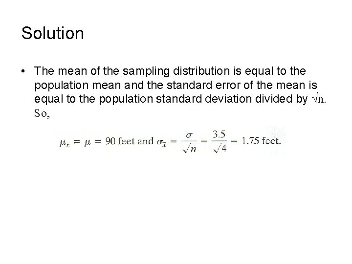
Solution • The mean of the sampling distribution is equal to the population mean and the standard error of the mean is equal to the population standard deviation divided by √n. So,

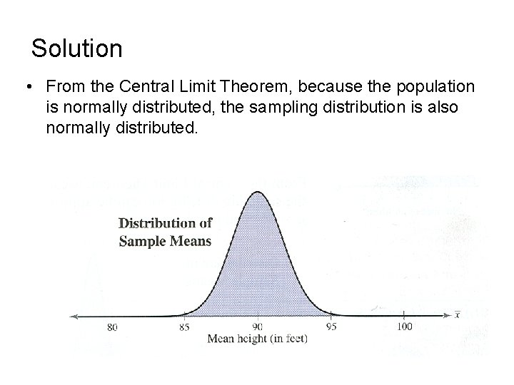
Solution • From the Central Limit Theorem, because the population is normally distributed, the sampling distribution is also normally distributed.

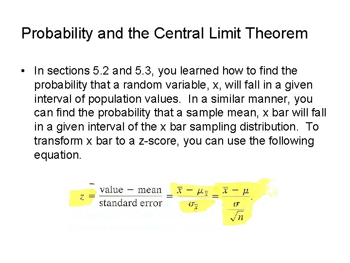
Probability and the Central Limit Theorem • In sections 5. 2 and 5. 3, you learned how to find the probability that a random variable, x, will fall in a given interval of population values. In a similar manner, you can find the probability that a sample mean, x bar will fall in a given interval of the x bar sampling distribution. To transform x bar to a z-score, you can use the following equation.

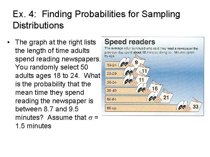
Ex. 4: Finding Probabilities for Sampling Distributions • The graph at the right lists the length of time adults spend reading newspapers. You randomly select 50 adults ages 18 to 24. What is the probability that the mean time they spend reading the newspaper is between 8. 7 and 9. 5 minutes? Assume that = 1. 5 minutes

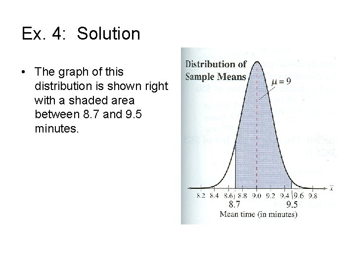
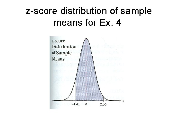
Ex. 4: Solution • The graph of this distribution is shown right with a shaded area between 8. 7 and 9. 5 minutes.

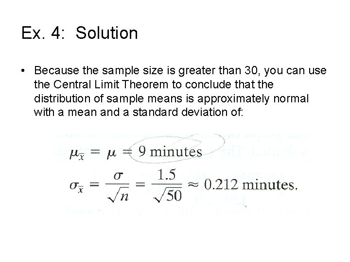
Ex. 4: Solution • Because the sample size is greater than 30, you can use the Central Limit Theorem to conclude that the distribution of sample means is approximately normal with a mean and a standard deviation of:

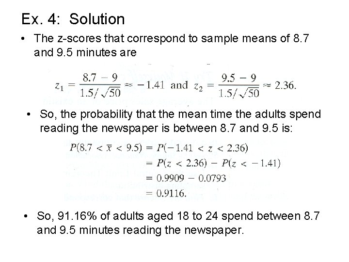
Ex. 4: Solution • The z-scores that correspond to sample means of 8. 7 and 9. 5 minutes are • So, the probability that the mean time the adults spend reading the newspaper is between 8. 7 and 9. 5 is: • So, 91. 16% of adults aged 18 to 24 spend between 8. 7 and 9. 5 minutes reading the newspaper.

z-score distribution of sample means for Ex. 4

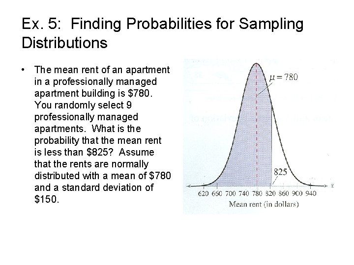
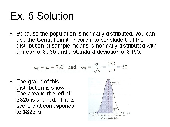
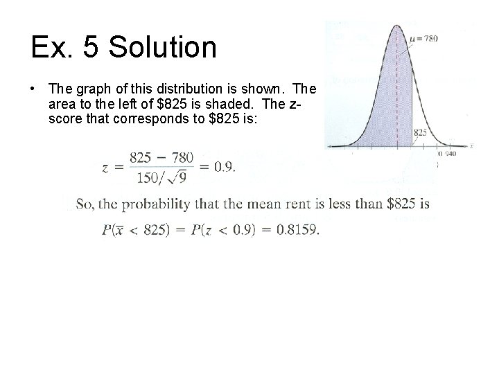
Ex. 5: Finding Probabilities for Sampling Distributions • The mean rent of an apartment in a professionally managed apartment building is $780. You randomly select 9 professionally managed apartments. What is the probability that the mean rent is less than $825? Assume that the rents are normally distributed with a mean of $780 and a standard deviation of $150.

Ex. 5 Solution • Because the population is normally distributed, you can use the Central Limit Theorem to conclude that the distribution of sample means is normally distributed with a mean of $780 and a standard deviation of $150. • The graph of this distribution is shown. The area to the left of $825 is shaded. The zscore that corresponds to $825 is:

Ex. 5 Solution • The graph of this distribution is shown. The area to the left of $825 is shaded. The zscore that corresponds to $825 is:

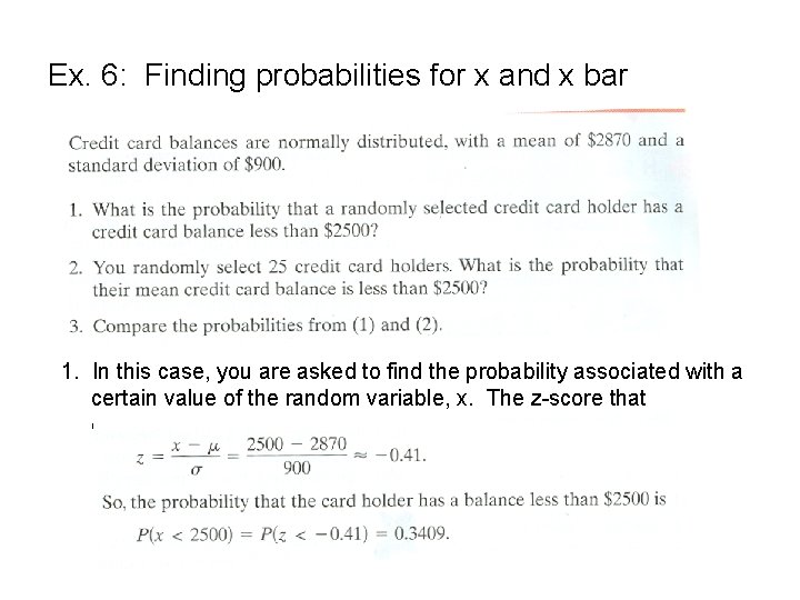
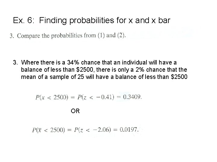
Ex. 6: Finding probabilities for x and x bar 1. In this case, you are asked to find the probability associated with a certain value of the random variable, x. The z-score that corresponds to x = $2500 is

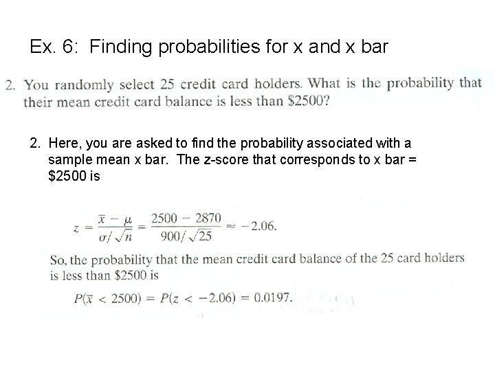
Ex. 6: Finding probabilities for x and x bar 2. Here, you are asked to find the probability associated with a sample mean x bar. The z-score that corresponds to x bar = $2500 is

Ex. 6: Finding probabilities for x and x bar 3. Where there is a 34% chance that an individual will have a balance of less than $2500, there is only a 2% chance that the mean of a sample of 25 will have a balance of less than $2500 OR