Introduction to Artificial Intelligence Unit 3 Constraint Satisfaction

Introduction to Artificial Intelligence – Unit 3 Constraint Satisfaction Problems Adversarial Search, Games Course 67842 The Hebrew University of Jerusalem School of Engineering and Computer Science Instructor: Jeff Rosenschein (Chapters 5 and 6, “Artificial Intelligence: A Modern Approach”)

Outline � Constraint Satisfaction Problems (CSP) � Backtracking search for CSPs � Problem Structure and Problem Decomposition � Local search for CSPs 2

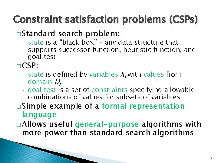
Constraint satisfaction problems (CSPs) � Standard search problem: ◦ state is a “black box” – any data structure that supports successor function, heuristic function, and goal test � CSP: ◦ state is defined by variables Xi with values from domain Di ◦ goal test is a set of constraints specifying allowable combinations of values for subsets of variables � Simple example of a formal representation language � Allows useful general-purpose algorithms with more power than standard search algorithms 3

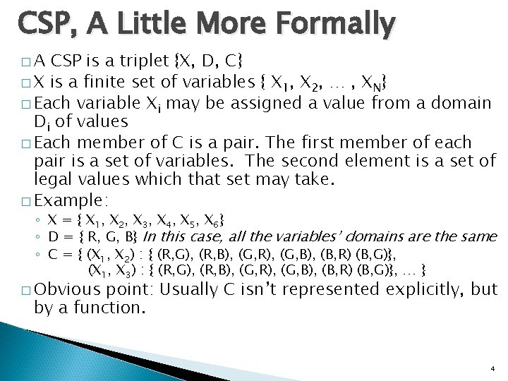
CSP, A Little More Formally �A CSP is a triplet {X, D, C} � X is a finite set of variables { X 1, X 2, … , XN} � Each variable Xi may be assigned a value from a domain Di of values � Each member of C is a pair. The first member of each pair is a set of variables. The second element is a set of legal values which that set may take. � Example: ◦ X = { X 1, X 2, X 3, X 4, X 5, X 6} ◦ D = { R, G, B} In this case, all the variables’ domains are the same ◦ C = { (X 1, X 2) : { (R, G), (R, B), (G, R), (G, B), (B, R) (B, G)}, (X 1, X 3) : { (R, G), (R, B), (G, R), (G, B), (B, R) (B, G)}, … } � Obvious point: Usually C isn’t represented explicitly, but by a function. 4

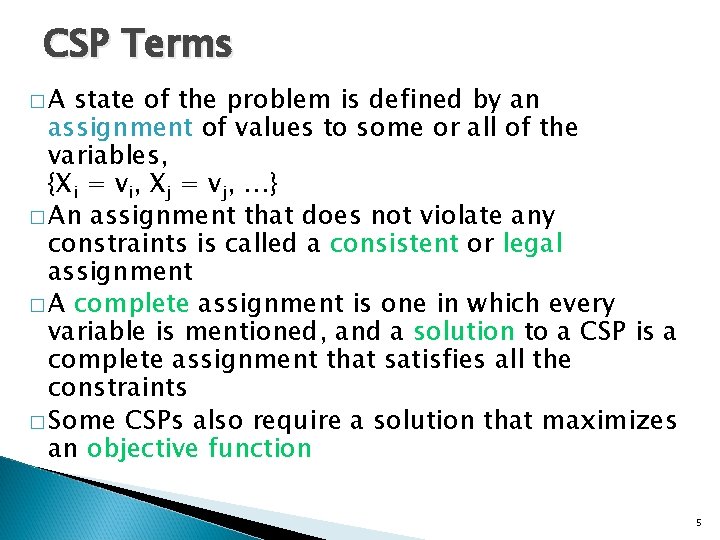
CSP Terms �A state of the problem is defined by an assignment of values to some or all of the variables, {Xi = vi, Xj = vj, …} � An assignment that does not violate any constraints is called a consistent or legal assignment � A complete assignment is one in which every variable is mentioned, and a solution to a CSP is a complete assignment that satisfies all the constraints � Some CSPs also require a solution that maximizes an objective function 5

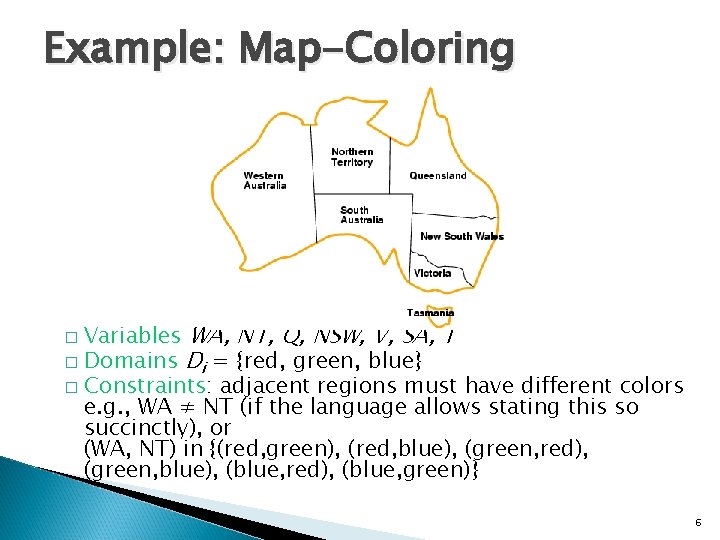
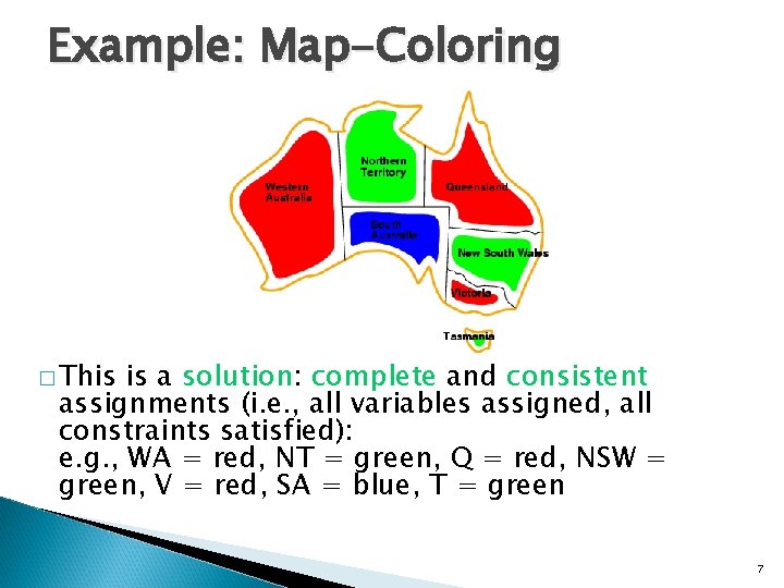
Example: Map-Coloring Variables WA, NT, Q, NSW, V, SA, T � Domains Di = {red, green, blue} � Constraints: adjacent regions must have different colors e. g. , WA ≠ NT (if the language allows stating this so succinctly), or (WA, NT) in {(red, green), (red, blue), (green, red), (green, blue), (blue, red), (blue, green)} � 6

Example: Map-Coloring � This is a solution: complete and consistent assignments (i. e. , all variables assigned, all constraints satisfied): e. g. , WA = red, NT = green, Q = red, NSW = green, V = red, SA = blue, T = green 7

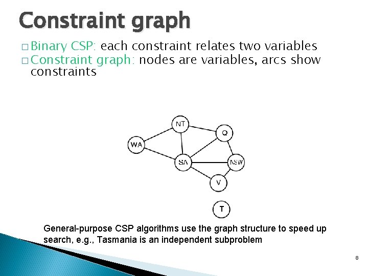
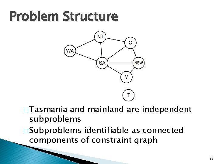
Constraint graph � Binary CSP: each constraint relates two variables � Constraint graph: nodes are variables, arcs show constraints General-purpose CSP algorithms use the graph structure to speed up search, e. g. , Tasmania is an independent subproblem 8

Varieties of CSPs �Discrete variables ◦ finite domains: �n variables, domain size d implies O(dn) complete assignments �e. g. , Boolean CSPs, including Boolean satisfiability (NP-complete) ◦ infinite domains: �integers, strings, etc. �e. g. , job scheduling, variables are start/end days for each job �need a constraint language, e. g. , Start. Job 1 + 5 ≤ Start. Job 3 �linear constraints solvable, nonlinear undecidable �Continuous variables ◦ e. g. , start/end times for Hubble Space Telescope observations ◦ linear constraints solvable in polynomial time by linear programming methods 9

Varieties of constraints �Unary constraints involve a single variable �Binary constraints involve pairs of variables ◦ e. g. , SA ≠ green ◦ e. g. , SA ≠ WA �Higher-order variables constraints involve 3 or more ◦ e. g. , cryptarithmetic column constraints �Preferences (soft constraints), e. g. , red is better than green, often representable by a cost for each variable assignment ◦ constrained optimization problems 10

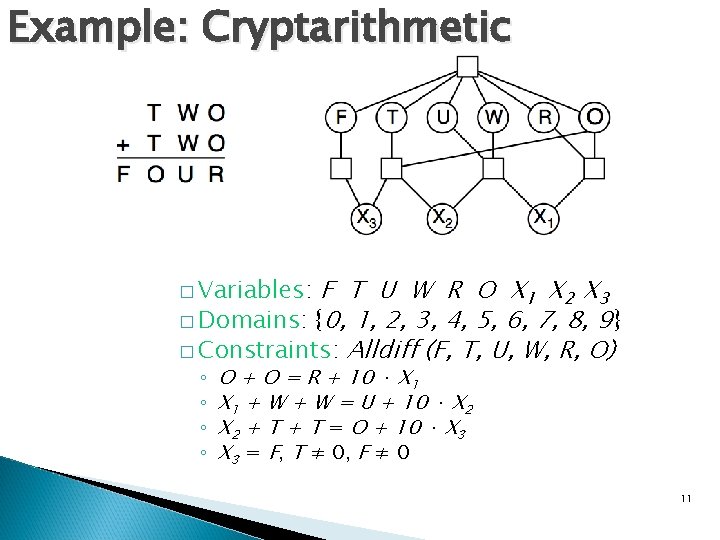
Example: Cryptarithmetic F T U W R O X 1 X 2 X 3 � Domains: {0, 1, 2, 3, 4, 5, 6, 7, 8, 9} � Constraints: Alldiff (F, T, U, W, R, O) � Variables: ◦ ◦ O + O = R + 10 · X 1 + W = U + 10 · X 2 + T = O + 10 · X 3 = F, T ≠ 0, F ≠ 0 11

Real-world CSPs �Assignment problems �Timetabling problems ◦ e. g. , who teaches what class? ◦ e. g. , which class (or exam) is offered when and where? �Hardware Configuration �Spreadsheets �Transportation scheduling �Factory scheduling �Floorplanning �Notice that many real-world problems involve real-valued variables 12

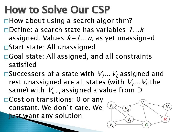
How to Solve Our CSP �How about using a search algorithm? �Define: a search state has variables 1…k assigned. Values k+1…n, as yet unassigned �Start state: All unassigned �Goal state: All assigned, and all constraints satisfied �Successors of a state with V 1…Vk assigned and rest unassigned are all states (with V 1…Vk the same) with Vk+1 assigned a value from D �Cost on transitions: 0 or any constant. We don’t care. We just want any solution. 13

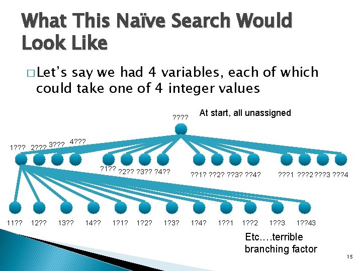
Standard search formulation (incremental) Let’s start with the straightforward (dumb) approach, then fix it. States are defined by the values assigned so far. � Initial state: the empty assignment { } � Successor function: assign a value to an unassigned variable that does not conflict with current assignment fail if no legal assignments � 1. 2. 3. 4. Goal test: the current assignment is complete This is the same for all CSPs (good) Every solution appears at depth n with n variables use depth-first search Path is irrelevant, so can also use complete-state formulation b = (n - l )d at depth l, hence n! · dn leaves (bad) b is branching factor, d is size of domain, n is number of variables 14

What This Naïve Search Would Look Like � Let’s say we had 4 variables, each of which could take one of 4 integer values ? ? At start, all unassigned 4? ? ? 1? ? ? 2? ? ? 3? ? ? 4? ? 11? ? 12? ? 13? ? 14? ? 1? 1? 2? 1? 3? ? ? 1? ? ? 2? ? ? 3? ? ? 4? 1? ? 1 1? ? 2 ? ? ? 1 ? ? ? 2 ? ? ? 3 ? ? ? 4 1? ? 3 1? ? 43 Etc. …terrible branching factor 15

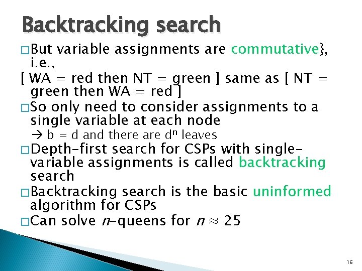
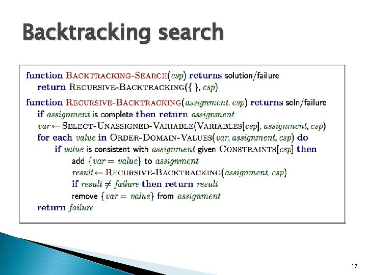
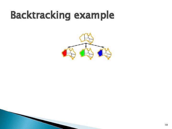
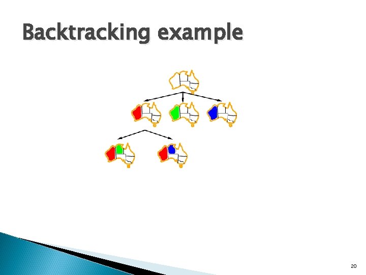
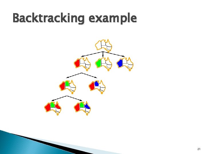
Backtracking search �But variable assignments are commutative}, i. e. , [ WA = red then NT = green ] same as [ NT = green then WA = red ] �So only need to consider assignments to a single variable at each node b = d and there are dn leaves �Depth-first search for CSPs with singlevariable assignments is called backtracking search �Backtracking search is the basic uninformed algorithm for CSPs �Can solve n-queens for n ≈ 25 16

Backtracking search 17

Backtracking example 18

Backtracking example 19

Backtracking example 20

Backtracking example 21

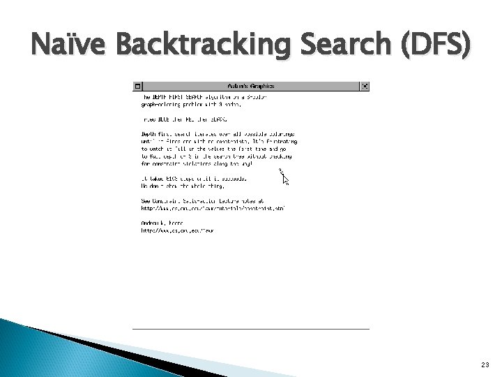
Animation – uninformed Backtracking (DFS) � http: //www. cs. cmu. edu/~awm/animations/constraint/9 d. htm l Tries Blue, then Red, then Black Does not do very well… 22

Naïve Backtracking Search (DFS) 23

Obvious Improvement � Don’t try successor that causes inconsistency with its neighbors � Backtracking still doesn’t look too good � http: //www. cs. cmu. edu/~awm/animations/c onstraint/9 b. html � http: //www. cs. cmu. edu/~awm/animations/c onstraint/27 b. html 24

Slightly better Backtracking (DFS) 25

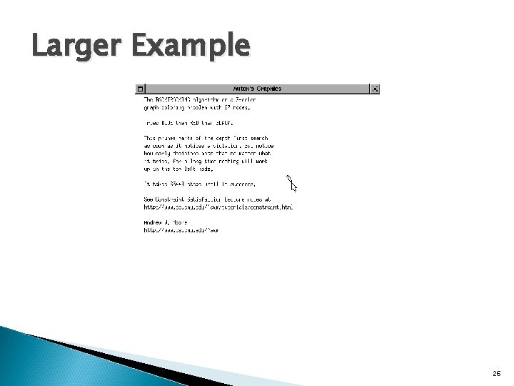
Larger Example 26

Backtracking search 27

Improving backtracking efficiency �General-purpose methods can give huge gains in speed: ◦ Which variable should be assigned next? ◦ In what order should its values be tried? ◦ Can we detect inevitable failure early? ◦ Can we take advantage of problem structure? 28

Improving backtracking efficiency �General-purpose methods can give huge gains in speed: ◦ Which variable should be assigned next? - Select. Unassigned. Variable ◦ In what order should its values be tried? - Order. Domain. Variables ◦ Can we detect inevitable failure early? ◦ Can we take advantage of problem structure? 29

Improving backtracking efficiency �General-purpose methods can give huge gains in speed: ◦ Which variable should be assigned next? ◦ In what order should its values be tried? ◦ Can we detect inevitable failure early? ◦ Can we take advantage of problem structure? 30

Minimum Remaining Values � Minimum remaining values (MRV): choose the variable with the fewest legal values All are the same here Two equivalent ones here Clear choice 31

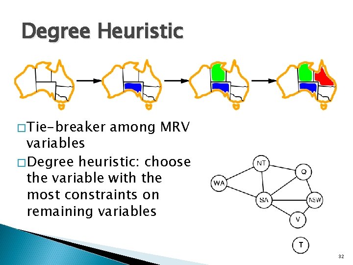
Degree Heuristic �Tie-breaker among MRV variables �Degree heuristic: choose the variable with the most constraints on remaining variables 32

Improving backtracking efficiency 33

Improving backtracking efficiency �General-purpose methods can give huge gains in speed: ◦ Which variable should be assigned next? ◦ In what order should its values be tried? ◦ Can we detect inevitable failure early? ◦ Can we take advantage of problem structure? 34

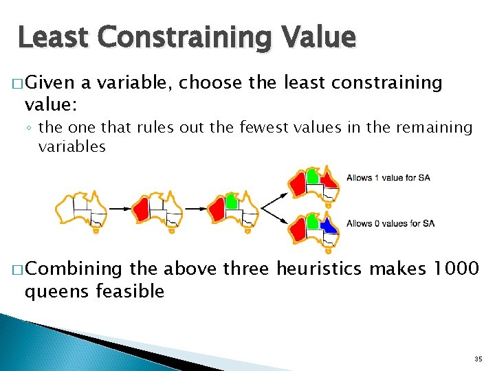
Least Constraining Value � Given value: a variable, choose the least constraining ◦ the one that rules out the fewest values in the remaining variables � Combining the above three heuristics makes 1000 queens feasible 35

Improving backtracking efficiency �General-purpose methods can give huge gains in speed: ◦ Which variable should be assigned next? ◦ In what order should its values be tried? �Least Constraining Value 36

Improving backtracking efficiency �General-purpose methods can give huge gains in speed: ◦ Which variable should be assigned next? ◦ In what order should its values be tried? ◦ Can we detect inevitable failure early? ◦ Can we take advantage of problem structure? 37

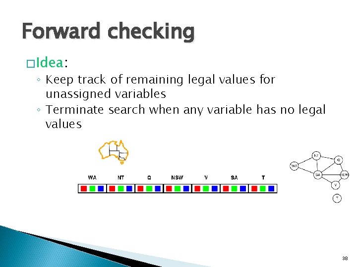
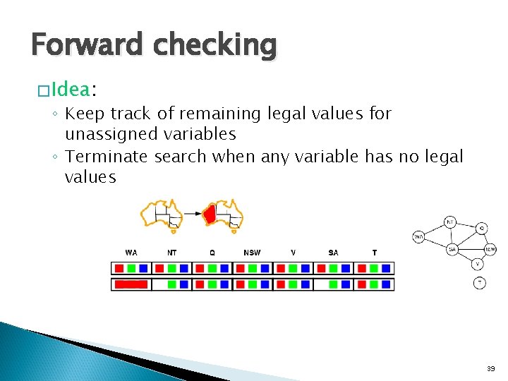
Forward checking �Idea: ◦ Keep track of remaining legal values for unassigned variables ◦ Terminate search when any variable has no legal values 38

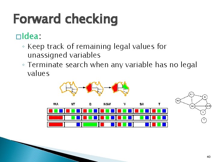
Forward checking �Idea: ◦ Keep track of remaining legal values for unassigned variables ◦ Terminate search when any variable has no legal values 39

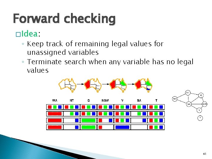
Forward checking �Idea: ◦ Keep track of remaining legal values for unassigned variables ◦ Terminate search when any variable has no legal values 40

Forward checking �Idea: ◦ Keep track of remaining legal values for unassigned variables ◦ Terminate search when any variable has no legal values 41

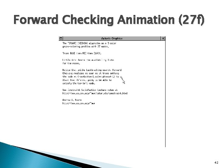
Forward Checking Animation (27 f) 42

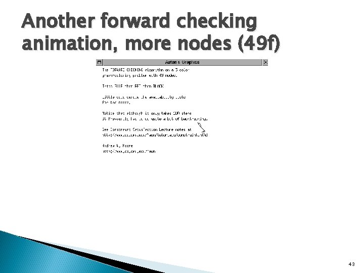
Another forward checking animation, more nodes (49 f) 43

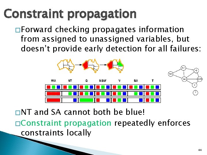
Constraint propagation �Forward checking propagates information from assigned to unassigned variables, but doesn’t provide early detection for all failures: �NT and SA cannot both be blue! �Constraint propagation repeatedly enforces constraints locally 44

Constraint Propagation �Forward checking computes the domain of each variable independently at the start, and then only updates these domains when assignments are made in the DFS that are directly relevant to the current variable. �Constraint Propagation carries this further. When you delete a value from your domain, check all variables connected to you. If any of them change, delete all inconsistent values connected to them, etc… 45

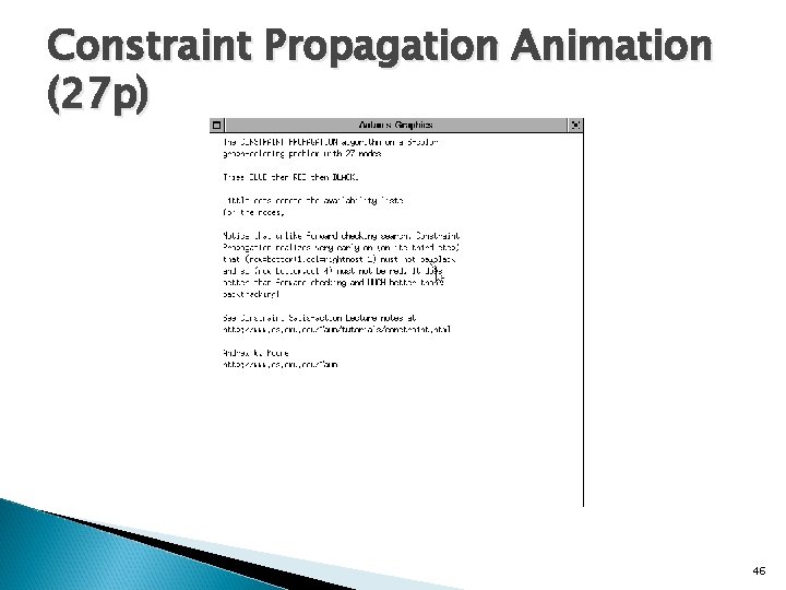
Constraint Propagation Animation (27 p) 46

Another constraint propagation animation, more nodes (49 p) 47

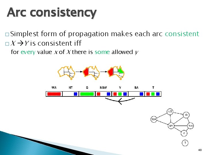
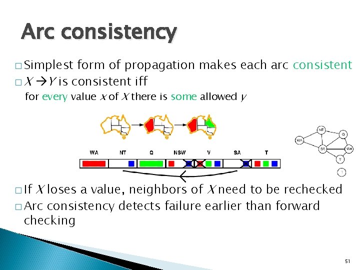
Arc consistency � Simplest form of propagation makes each arc consistent � X Y is consistent iff for every value x of X there is some allowed y 48

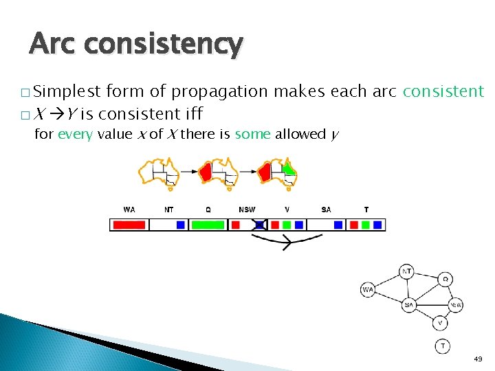
Arc consistency � Simplest form of propagation makes each arc consistent � X Y is consistent iff for every value x of X there is some allowed y 49

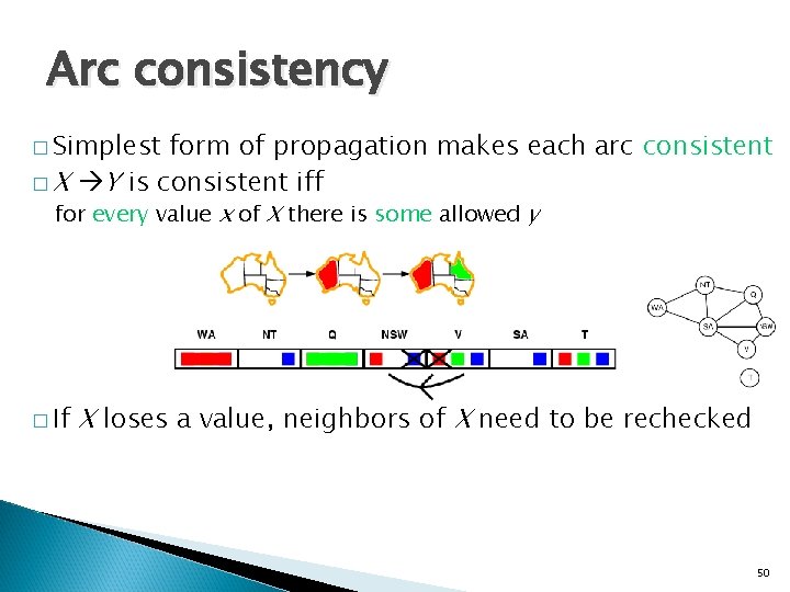
Arc consistency � Simplest form of propagation makes each arc consistent � X Y is consistent iff for every value x of X there is some allowed y � If X loses a value, neighbors of X need to be rechecked 50

Arc consistency � Simplest form of propagation makes each arc consistent � X Y is consistent iff for every value x of X there is some allowed y � If X loses a value, neighbors of X need to be rechecked � Arc consistency detects failure earlier than forward checking 51

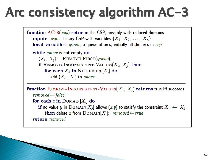
Arc consistency algorithm AC-3 52

Improving backtracking efficiency �General-purpose methods can give huge gains in speed: ◦ Which variable should be assigned next? ◦ In what order should its values be tried? ◦ Can we detect inevitable failure early? �Forward Checking �Constraint Propagation �Arc Consistency 53

Improving backtracking efficiency �General-purpose methods can give huge gains in speed: ◦ Which variable should be assigned next? ◦ In what order should its values be tried? ◦ Can we detect inevitable failure early? ◦ Can we take advantage of problem structure? 54

Problem Structure � Tasmania and mainland are independent subproblems � Subproblems identifiable as connected components of constraint graph 55

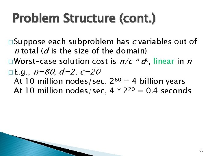
Problem Structure (cont. ) each subproblem has c variables out of n total (d is the size of the domain) � Worst-case solution cost is n/c * dc, linear in n � E. g. , n=80, d=2, c=20 At 10 million nodes/sec, 280 = 4 billion years At 10 million nodes/sec, 4 * 220 = 0. 4 seconds � Suppose 56

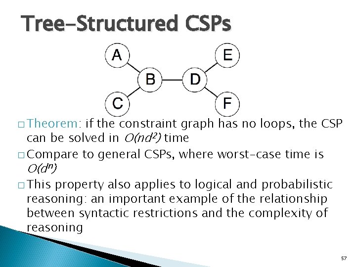
Tree-Structured CSPs � Theorem: if the constraint graph has no loops, the CSP can be solved in O(nd 2) time � Compare to general CSPs, where worst-case time is O(dn) � This property also applies to logical and probabilistic reasoning: an important example of the relationship between syntactic restrictions and the complexity of reasoning 57

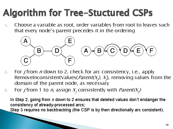
Algorithm for Tree-Stuctured CSPs 1. 2. 3. Choose a variable as root, order variables from root to leaves such that every node’s parent precedes it in the ordering For j from n down to 2, check for arc consistency, i. e. , apply Remove. Inconsistent. Values(Parent(Xj), removing values from the domain of the parent node, as necessary For j from 1 to n, assign Xj consistently with Parent(Xj) In Step 2, going from n down to 2 ensures that deleted values don’t endanger the consistency of already-processed arcs; Step 3 requires no backtracking (the CSP is by then directionally arc consistent). 58

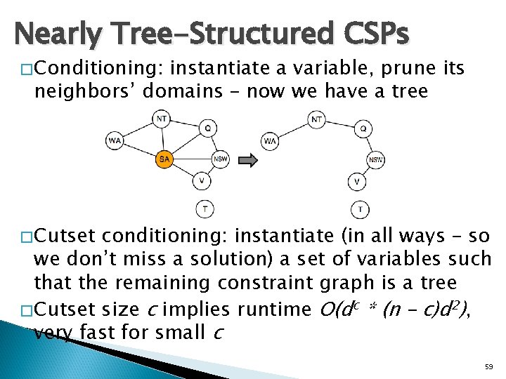
Nearly Tree-Structured CSPs �Conditioning: instantiate a variable, prune its neighbors’ domains – now we have a tree �Cutset conditioning: instantiate (in all ways – so we don’t miss a solution) a set of variables such that the remaining constraint graph is a tree �Cutset size c implies runtime O(dc * (n – c)d 2), very fast for small c 59

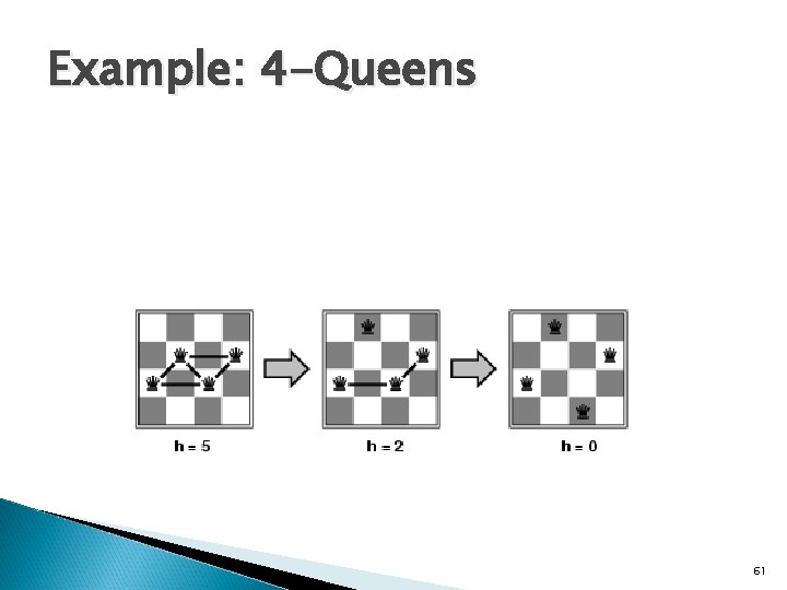
Iterative Algorithms for CSPs �Hill-climbing, simulated annealing typically work with “complete” states, i. e. , all variables assigned �To apply to CSPs: ◦ use complete states, but with unsatisfied constraints ◦ operators reassign variable values �Variable selection: randomly select any conflicted variable �Value selection by min-conflicts heuristic: ◦ choose value that violates the fewest constraints ◦ i. e. , hill-climb with h(n) = total number of violated constraints 60

Example: 4 -Queens 61

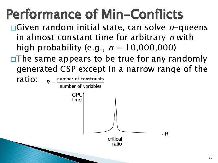
Performance of Min-Conflicts random initial state, can solve n-queens in almost constant time for arbitrary n with high probability (e. g. , n = 10, 000) �The same appears to be true for any randomly generated CSP except in a narrow range of the ratio: �Given 62

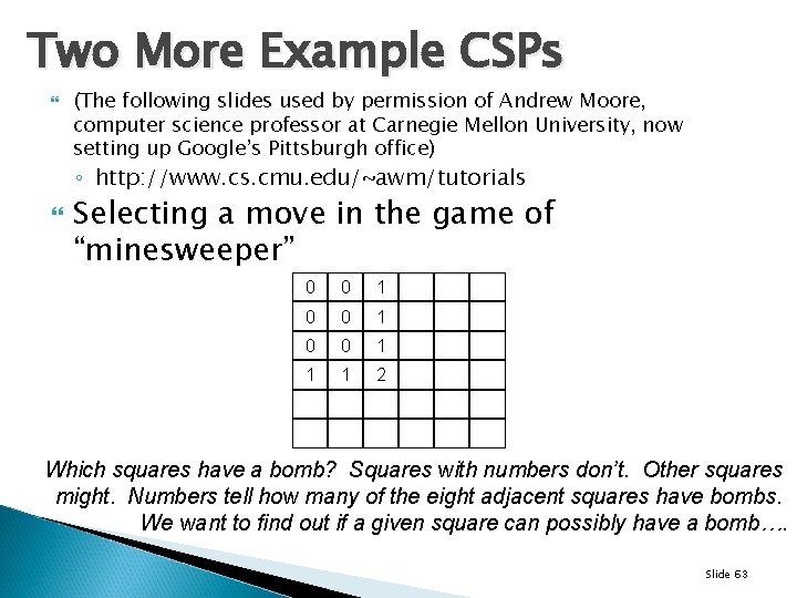
Two More Example CSPs (The following slides used by permission of Andrew Moore, computer science professor at Carnegie Mellon University, now setting up Google’s Pittsburgh office) ◦ http: //www. cs. cmu. edu/~awm/tutorials Selecting a move in the game of “minesweeper” 0 0 1 1 1 2 Which squares have a bomb? Squares with numbers don’t. Other squares might. Numbers tell how many of the eight adjacent squares have bombs. We want to find out if a given square can possibly have a bomb…. Slide 63

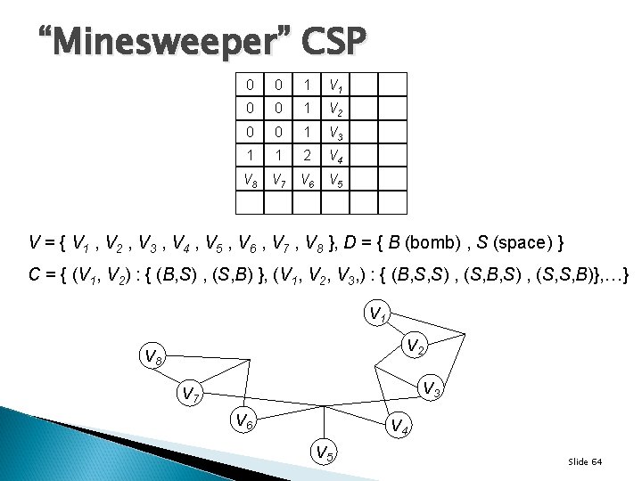
“Minesweeper” CSP 0 0 1 V 1 0 0 1 V 2 0 0 1 V 3 1 1 2 V 4 V 8 V 7 V 6 V 5 V = { V 1 , V 2 , V 3 , V 4 , V 5 , V 6 , V 7 , V 8 }, D = { B (bomb) , S (space) } C = { (V 1, V 2) : { (B, S) , (S, B) }, (V 1, V 2, V 3, ) : { (B, S, S) , (S, B, S) , (S, S, B)}, …} V 1 V 2 V 8 V 3 V 7 V 6 V 4 V 5 Slide 64

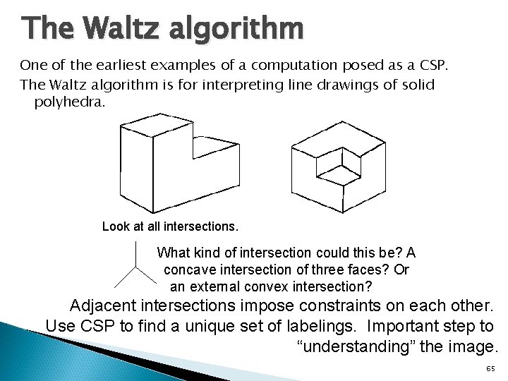
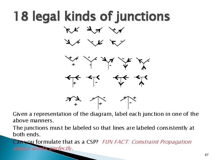
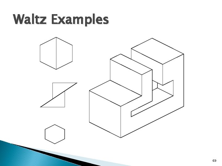
The Waltz algorithm One of the earliest examples of a computation posed as a CSP. The Waltz algorithm is for interpreting line drawings of solid polyhedra. Look at all intersections. What kind of intersection could this be? A concave intersection of three faces? Or an external convex intersection? Adjacent intersections impose constraints on each other. Use CSP to find a unique set of labelings. Important step to “understanding” the image. 65

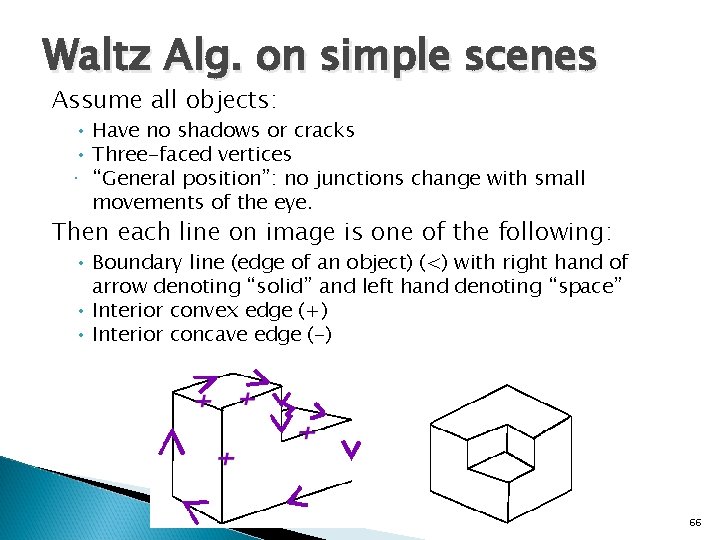
Waltz Alg. on simple scenes Assume all objects: • Have no shadows or cracks • Three-faced vertices • “General position”: no junctions change with small movements of the eye. Then each line on image is one of the following: • Boundary line (edge of an object) (<) with right hand of arrow denoting “solid” and left hand denoting “space” • Interior convex edge (+) • Interior concave edge (-) 66

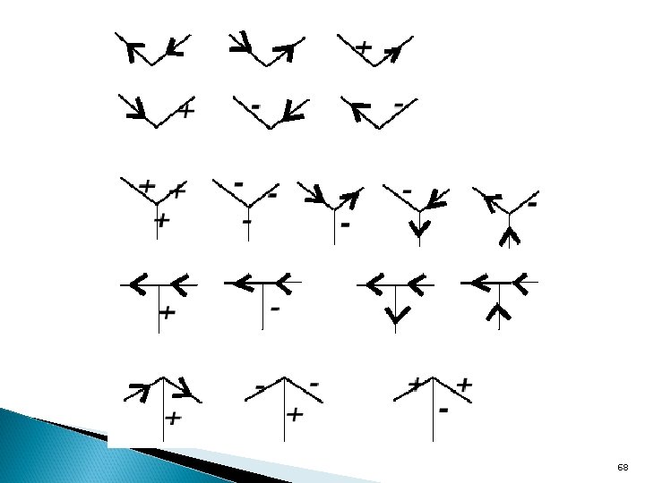
18 legal kinds of junctions Given a representation of the diagram, label each junction in one of the above manners. The junctions must be labeled so that lines are labeled consistently at both ends. Can you formulate that as a CSP? FUN FACT: Constraint Propagation always works perfectly. 67

68

Waltz Examples 69

Summary � CSPs are a special kind of search problem: ◦ states defined by values of a fixed set of variables ◦ goal test defined by constraints on variable values � Backtracking = depth-first search with one variable assigned per node � Variable ordering (MRV, degree heuristic) and value selection (least constraining value) heuristics help significantly � Forward checking prevents assignments that guarantee later failure � Constraint propagation (e. g. , arc consistency) does additional work to constrain values and detect inconsistencies � The CSP representation allows analysis of problem structure � Tree-structured CSPs can be solved in linear time � Iterative min-conflicts is usually effective in practice 70

Adversarial Search Chapter 5 Sections 1 – 4, 6

Outline � Games � Perfect Play ◦ minimax decisions ◦ α-β pruning � Resource limits and approximate evaluation � Games of chance � Games of imperfect information 72

Games vs. search problems opponent solution is a strategy, specifying a move for every possible opponent reply � Time limits unlikely to find goal, must approximate � Plan of attack: � “Unpredictable” ◦ Computer considers all lines of play (Babbage, 1846) ◦ Algorithm for perfect play (Zermolo, 1912; Von Neumann, 1944) ◦ Finite horizon, approximate evaluation (Zuse, 1945; Wiener, 1948; Shannon, 1950) ◦ First chess program (Turing, 1951) ◦ Machine learning to improve evaluation accuracy (Samuel, 19521957) ◦ Pruning to allow deeper search (Mc. Carthy, 1956) 73

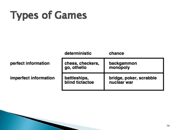
Types of Games 74

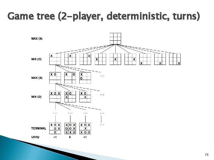
Game tree (2 -player, deterministic, turns) 75

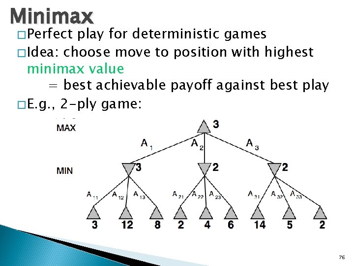
Minimax �Perfect play for deterministic games �Idea: choose move to position with highest minimax value = best achievable payoff against best play �E. g. , 2 -ply game: 76

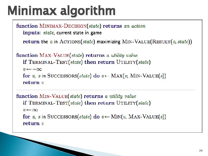
Minimax algorithm 77

Properties of minimax �Complete? Only if tree is finite (chess has specific rules for this); note that a finite strategy can exist even in an infinite tree �Optimal? Yes, against an optimal opponent; otherwise? �Time complexity? O(bm) (b = legal moves, m = maximum depth of tree) �Space complexity? O(bm) (depth-first exploration ◦ For chess, b ≈ 35, m ≈100 for “reasonable” games exact solution completely infeasible But do we need to explore every path? 78

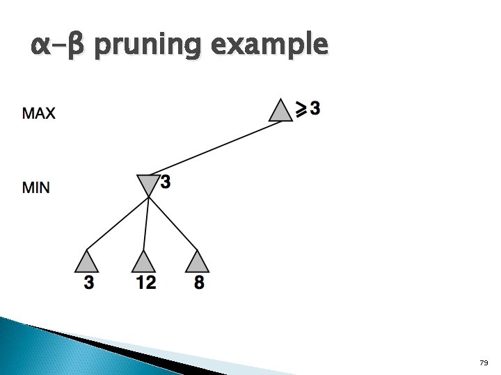
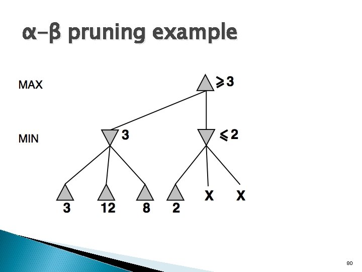
α-β pruning example 79

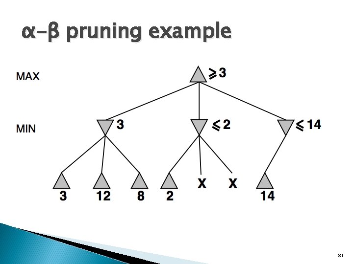
α-β pruning example 80

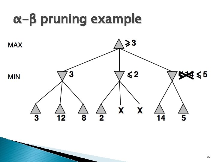
α-β pruning example 81

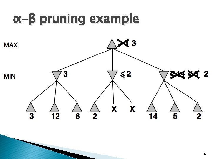
α-β pruning example 82

α-β pruning example 83

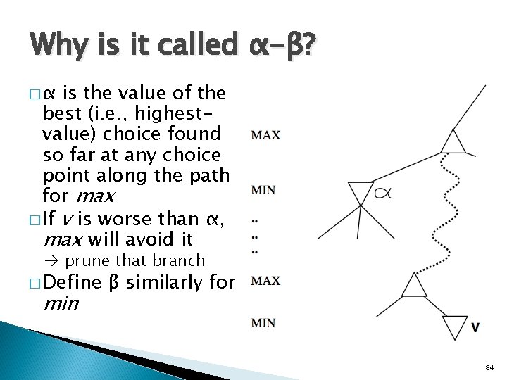
Why is it called α-β? �α is the value of the best (i. e. , highestvalue) choice found so far at any choice point along the path for max � If v is worse than α, max will avoid it prune that branch � Define min β similarly for 84

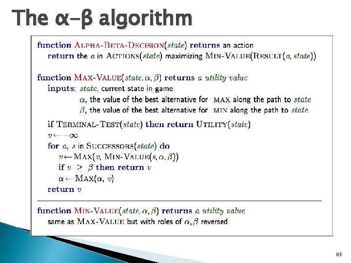
The α-β algorithm 85

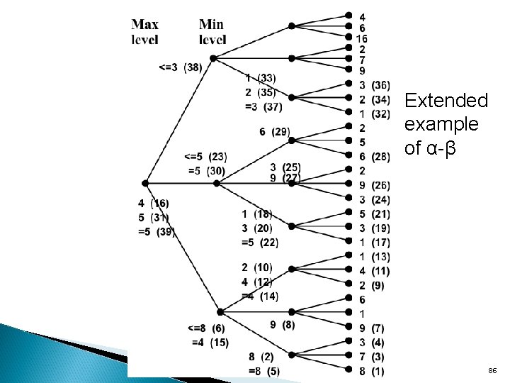
Extended example of α-β 86

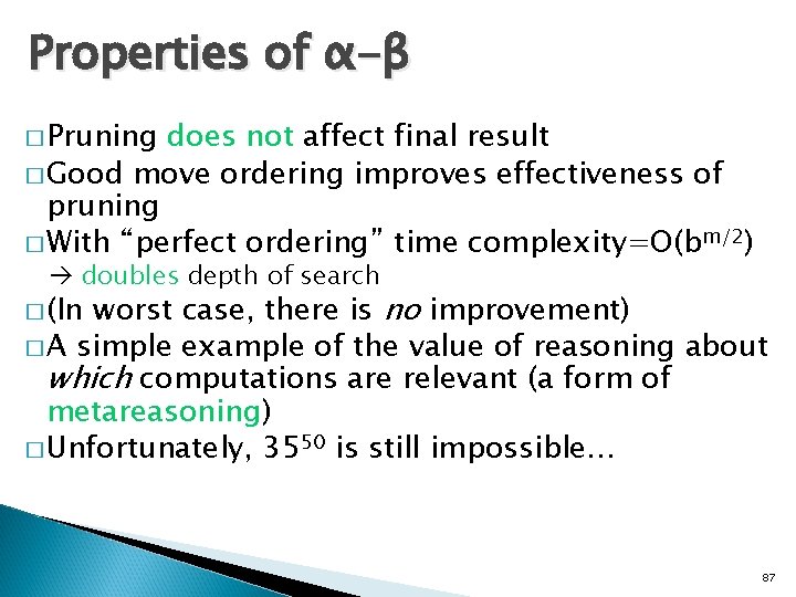
Properties of α-β � Pruning does not affect final result � Good move ordering improves effectiveness of pruning � With “perfect ordering” time complexity=O(bm/2) doubles depth of search worst case, there is no improvement) � A simple example of the value of reasoning about which computations are relevant (a form of metareasoning) � Unfortunately, 3550 is still impossible… � (In 87

Resource limits Standard approach: �Use Cutoff test instead of Terminal test: e. g. , depth limit (perhaps add quiescence search) �Use Eval instead of Utility ◦ i. e. , evaluation function that estimates desirability of position Suppose we have 100 seconds, explore 104 nodes/sec 106 nodes per move, approximately 358/2 � 4 -ply lookahead is a hopeless chess player! ◦ 4 -ply ≈ human novice ◦ 8 -ply ≈ mid-level PC, human master ◦ 12 -ply ≈ Deep Blue, Kasparov α-β reaches depth 8, i. e. , pretty good chess program 88

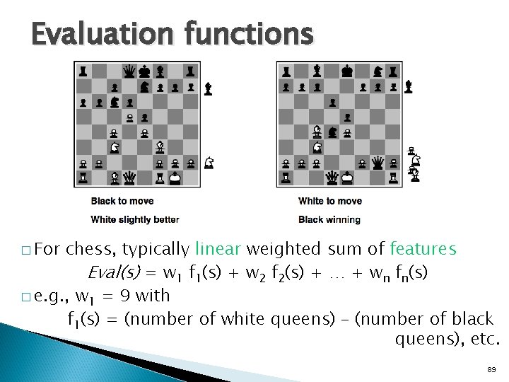
Evaluation functions � For chess, typically linear weighted sum of features Eval(s) = w 1 f 1(s) + w 2 f 2(s) + … + wn fn(s) � e. g. , w 1 = 9 with f 1(s) = (number of white queens) – (number of black queens), etc. 89

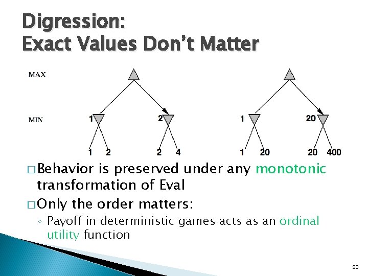
Digression: Exact Values Don’t Matter � Behavior is preserved under any monotonic transformation of Eval � Only the order matters: ◦ Payoff in deterministic games acts as an ordinal utility function 90

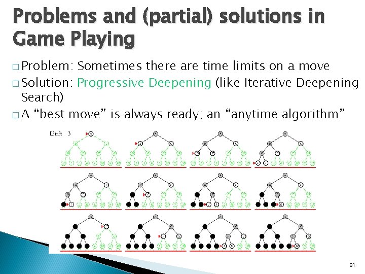
Problems and (partial) solutions in Game Playing � Problem: Sometimes there are time limits on a move � Solution: Progressive Deepening (like Iterative Deepening Search) � A “best move” is always ready; an “anytime algorithm” 91

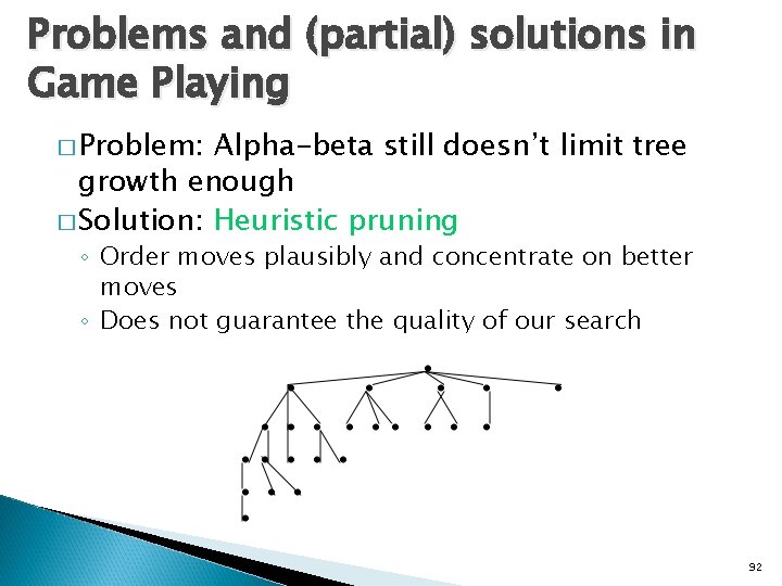
Problems and (partial) solutions in Game Playing � Problem: Alpha-beta still doesn’t limit tree growth enough � Solution: Heuristic pruning ◦ Order moves plausibly and concentrate on better moves ◦ Does not guarantee the quality of our search 92

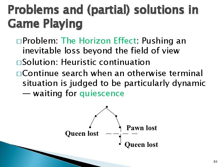
Problems and (partial) solutions in Game Playing � Problem: The Horizon Effect: Pushing an inevitable loss beyond the field of view � Solution: Heuristic continuation � Continue search when an otherwise terminal situation is judged to be particularly dynamic — waiting for quiescence 93

Other improvements in game search methods � Secondary search – check more deeply into a chosen move � Book moves – use a “table lookup” – sometimes is feasible (beginning or end of game) � Limitations of all these methods: ◦ Need to get a single number to reflect a position ◦ Assumption of opponent’s infallibility 94

Deterministic games in practice � Checkers: Chinook ended 40 -year-reign of human world champion Marion Tinsley in 1994. Used a precomputed endgame database defining perfect play for all positions involving 8 or fewer pieces on the board, a total of 443, 748, 401, 247 positions. � A precomputed endgame database? Would it be possible to extend the “endgame” all the way back to the beginning of the game, essentially “solving” checkers? 95

Checkers is Solved Originally published in Science Express on 19 July 2007 Science 14 September 2007: Vol. 317, no. 5844, pp. 1518 – 1522 Jonathan Schaeffer (University of Alberta), Neil Burch, Yngvi Björnsson, Akihiro Kishimoto, Martin Müller, Robert Lake, Paul Lu, Steve Sutphen The game of checkers has roughly 500 billion possible positions (5 x 1020). The task of solving the game, determining the final result in a game with no mistakes made by either player, is daunting. Since 1989, almost continuously, dozens of computers have been working on solving checkers, applying state-of-the-art artificial intelligence techniques to the proving process. This paper announces that checkers is now solved: Perfect play by both sides leads to a draw. This is the most challenging popular game to be solved to date, roughly one million times as complex as Connect Four. Artificial intelligence technology has been used to generate strong heuristicbased game-playing programs, such as Deep Blue for chess. Solving a game takes this to the next level by replacing the heuristics with perfection. 96

Deterministic games in practice � Chess: Deep Blue defeated human world champion Garry Kasparov in a six-game match in 1997. Deep Blue searches 200 million positions per second, uses very sophisticated evaluation, and undisclosed methods for extending some lines of search up to 40 ply. Rybka was the 2008 and 2009 computer chess champion (uses an off-the-shelf 8 -core 3. 2 GHz Intel Xeon processor), but was stripped of its titles for having plagiarized two other programs… � Othello: Logistello beats human world champion in 1997; human champions refuse to compete against computers, who are too good � Go: human champions refuse to compete against computers, who are too bad. In go, b > 300, so most programs use pattern knowledge bases to suggest plausible moves. 97

Summary � Games are fun to work on! � They illustrate several important points about AI ◦ ◦ Perfection is unattainable must approximate Good idea to think about what to think about Uncertainty constrains the assignment of values to states Optimal decisions depend on information state, not real state � Games are to AI as grand prix racing is to automobile design 98