Initial Value Problems Solution of Ordinary Differential Equations


 with initial conditions x(t")
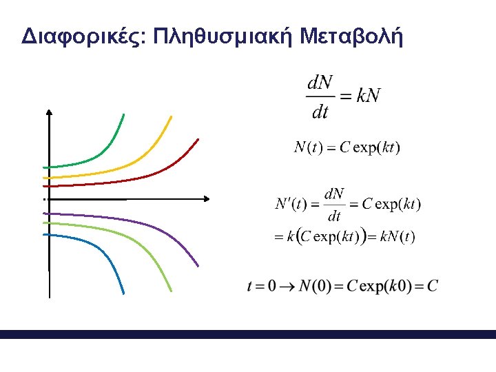
Initial Value Problems • Solution of Ordinary Differential Equations (ODEs) with initial conditions x(t 0) = x[0] at t 0 = 0. • Exact solution:
 with initial conditions x(t")
Initial Value Problems • Solution of Ordinary Differential Equations (ODEs) with initial conditions x(t 0) = x[0]. • Solution:

Solution of a Single ODE • Single step • Multistep • Explicit • Implicit
 • General Single-step method • Euler’s fwd Method")
Fwd Euler’s Method (explicit/single-step) • General Single-step method • Euler’s fwd Method
 The idea is the same as for the fwd Euler")
Bwd Euler’s Method (implicit/single-step) The idea is the same as for the fwd Euler method with the only difference that the slope is estimate at t[k+1] instead for t[k] Unless the last equation is linear or quadratic, it has to be solved numerically.

Modified Euler & Midpoint Method • Modified Euler Method • Midpoint Method

Runge-Kutta Methods • Family of single-step explicit methods • Order: defines the number of points taken at the subinterval [t[k], t[k+1]] • 2 nd Order RK (RK-2)
")
3 rd Order Runge-Kutta Method (RK-3)
 Method c 1 c 2 c 3 a")
3 rd Order Runge-Kutta Method (RK-3) Method c 1 c 2 c 3 a 2 b 21 a 3 b 31 b 32 Classical 1/6 4/6 1/2 1 -1 2 Nystrom’s 2/8 3/8 2/3 2/3 0 2/3 Nearly Optimal 2/9 3/9 4/9 1/2 3/4 0 3/4 Heun’s Third 1/4 0 3/4 1/3 2/3 0 2/3
 c 1 c 2 c 3 c 4")
4 th Order Runge-Kutta Method (RK-4) c 1 c 2 c 3 c 4 a 2 a 3 a 4 b 21 b 32 b 41 b 42 b 43 1/6 2/6 1/2 1 1/2 0 0 1

Multistep Methods • General form • Adams-Bashforth

Linear ODE Systems • System of linear first-order ODEs
 • Solution of the system: • Time marching")
ODE Solvers: Single-step Implicit (Time marching) • Solution of the system: • Time marching solvers Update x(t) in discrete time steps h = Δt approx.
 • Explicit single-step (forward) Euler method yields: •")
ODE Solvers: Single-step Explicit (Time marching) • Explicit single-step (forward) Euler method yields: • Because this method is not very accurate we usually apply the 4 th-order Runge-Kutta (RK 4) method:
 • Implicit (backward) Euler method • Crank-Nicholson method")
ODE Solvers: Single-step Implicit (Time marching) • Implicit (backward) Euler method • Crank-Nicholson method (modified Euler method)

Initial Value Problems • Reaction kinetics
. function f")
MATLAB ODE solvers • Use of the function ode 45 (Explicit Method). function f = batch_reactor_ex_calc_f(t, x, k 1, k 2); f = zeros(size(x)); % extract concentrations from state vector c. A = x(1); c. B = x(2); c. C = x(3); c. D = x(4); % compute rates of each reaction r 1 = k 1*c. A*c. B; r 2 = k 2*c. C*c. B; f(1) = -r 1; % mole balance on A f(2) = -r 1 -r 2; % mole balance on B f(3) = r 1 - r 2; % mole balance on C f(4) = r 2; % mole balance on D return;
. % set")
MATLAB ODE solvers • Use of the function ode 45 (Explicit Method). % set initial state c. A 0 = 1; c. B 0 = 2; x 0 = [c. A 0; c. B 0; 0; 0]; k 1 = 1; k 2 = 0. 5; % set fixed parameters T_end = 10; % set end time % call ode 45 to perform simulation [t_traj, x_traj] = ode 45(@batch_reactor_ex_calc_f, . . . [0 t_end], x 0, [ ], k 1, k 2); % plot results figure; plot(t_traj, x_traj(: , 1)); hold on; plot(t traj, x_traj(: , 2), ‘--’); plot(t_traj, x_traj(: , 3), ‘-. ’); plot(t_traj, x_traj(: , 4), ‘: ’);

MATLAB ODE solvers
. Estimate")
MATLAB ODE solvers • Use of the function ode 15 s (Implicit Method). Estimate the Jacobian: Syntax

ODE Solvers: Stiffness • Consider the following reactions:

ODE Solvers: Stiffness • Estimation of the Jacobian: the eigenvalues are –k 1 c. M and –k 2

ODE Solvers: Stiffness k 1 c. M = 1, k 2 = 100

ODE Solvers: Stiffness

ODE Sovlers in Matlab Solver Description ode 45 Non-stiff problems. Apply as a first approach. Single-step method RK-4 and RK-5. ode 23 Non-stiff problems. Apply as a first approach. Single-step method RK-2 and RK-3. ode 113 Non-stiff problems. Multistep method. ode 15 s Stiff problems. Multistep method. ode 23 s Stiff problems. Single-step method.
- Slides: 29