LAPLACE TRANSFORMS INTRODUCTION Definition n Transforms a mathematical

LAPLACE TRANSFORMS INTRODUCTION

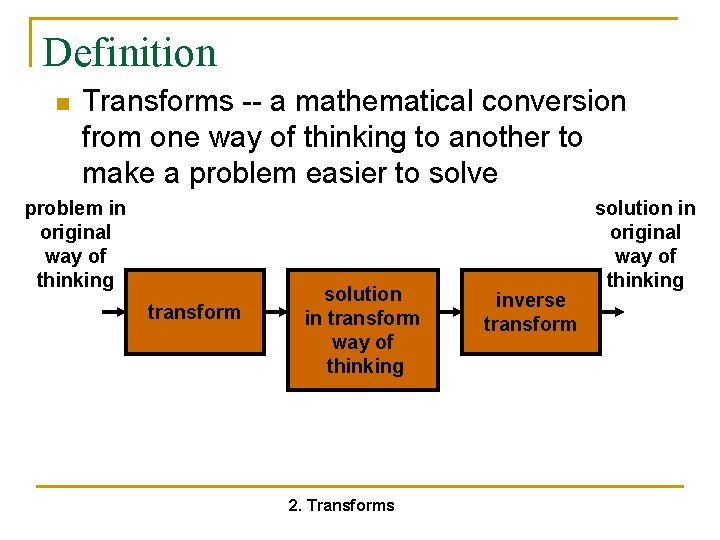
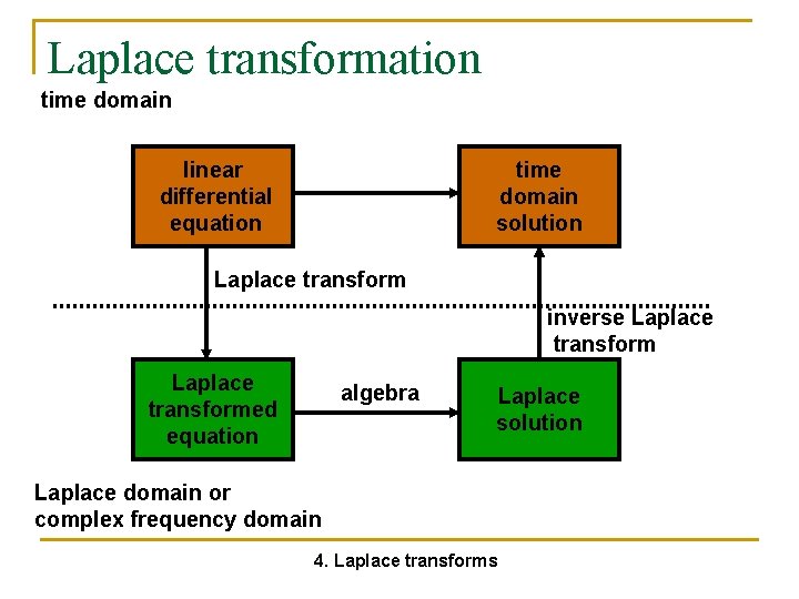
Definition n Transforms -- a mathematical conversion from one way of thinking to another to make a problem easier to solve problem in original way of thinking transform solution in transform way of thinking 2. Transforms inverse transform solution in original way of thinking

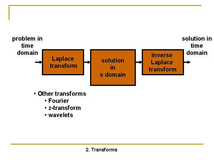
problem in time domain Laplace transform solution in s domain • Other transforms • Fourier • z-transform • wavelets 2. Transforms inverse Laplace transform solution in time domain

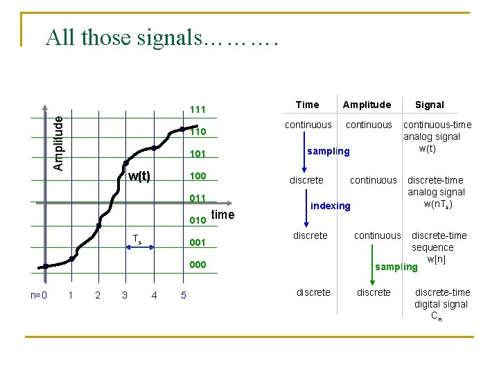
All those signals………. Amplitude 111 110 100 Ts 001 continuous discrete 011 010 Amplitude sampling 101 w(t) Time time indexing discrete 000 n=0 1 2 3 4 5 continuous discrete Signal continuous-time analog signal w(t) discrete-time analog signal w(n. Ts) continuous discrete-time sequence w[n] sampling discrete-time digital signal Cn

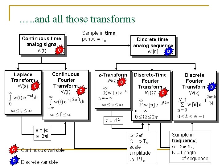
…. . and all those transforms Continuous-time analog signal C w(t) Laplace Transform W(s) C Sample in time, period = Ts Continuous Fourier Transform C W(f) z-Transform W(z) C Discrete-time analog sequence D w [n] Discrete-Time Fourier Transform W(W) C Discrete Fourier Transform D W(k) z = ej. W s = j =2 pf C Continuous-variable D Discrete-variable =2 pf W = Ts, scale amplitude by 1/Ts Sample in frequency, W = 2 pn/N, N = Length of sequence

Laplace transformation time domain linear differential equation time domain solution Laplace transform inverse Laplace transformed equation algebra Laplace solution Laplace domain or complex frequency domain 4. Laplace transforms

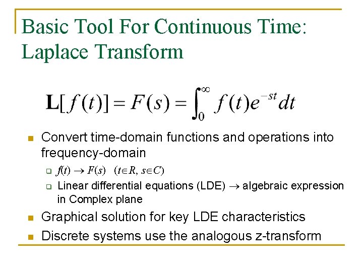
Basic Tool For Continuous Time: Laplace Transform n Convert time-domain functions and operations into frequency-domain q q n n f(t) ® F(s) (t R, s C) Linear differential equations (LDE) ® algebraic expression in Complex plane Graphical solution for key LDE characteristics Discrete systems use the analogous z-transform

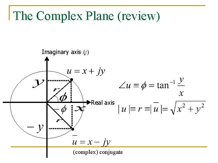
The Complex Plane (review) Imaginary axis (j) Real axis (complex) conjugate

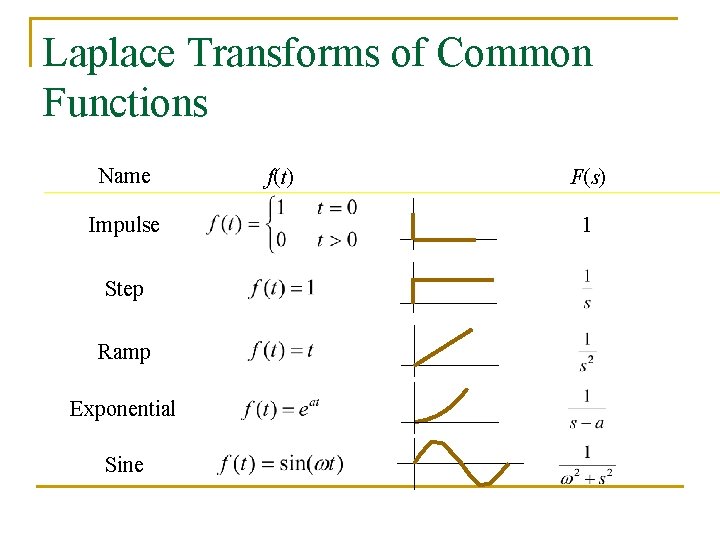
Laplace Transforms of Common Functions Name Impulse Step Ramp Exponential Sine f(t) F(s) 1

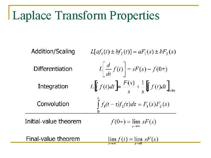
Laplace Transform Properties

LAPLACE TRANSFORMS SIMPLE TRANSFORMATIONS

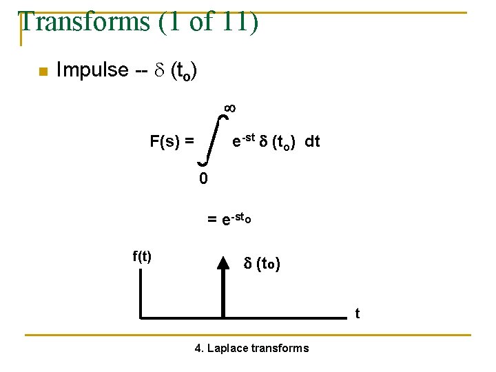
Transforms (1 of 11) n Impulse -- (to) e-st (to) dt F(s) = 0 = e-sto f(t) (to) t 4. Laplace transforms

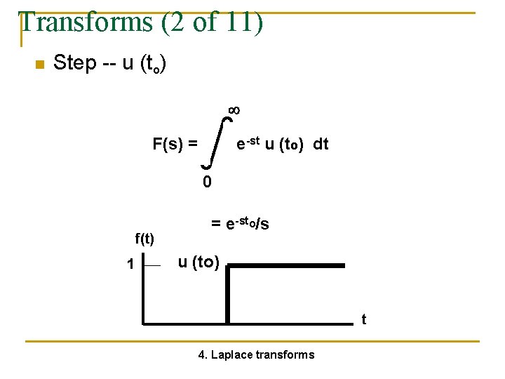
Transforms (2 of 11) n Step -- u (to) F(s) = e-st u (to) dt 0 f(t) 1 = e-sto/s u (to) t 4. Laplace transforms

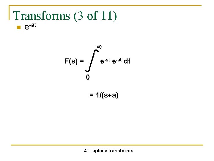
Transforms (3 of 11) n e-at F(s) = e-st e-at dt 0 = 1/(s+a) 4. Laplace transforms

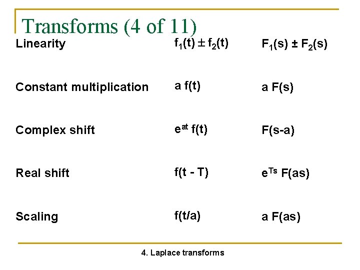
Transforms (4 of 11) Linearity f 1(t) f 2(t) F 1(s) ± F 2(s) Constant multiplication a f(t) a F(s) Complex shift eat f(t) F(s-a) Real shift f(t - T) e. Ts F(as) Scaling f(t/a) a F(as) 4. Laplace transforms

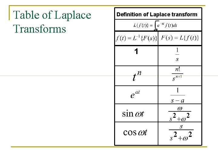
Transforms (5 of 11) n Most mathematical handbooks have tables of Laplace transforms 4. Laplace transforms

Table of Laplace Transforms Definition of Laplace transform 1

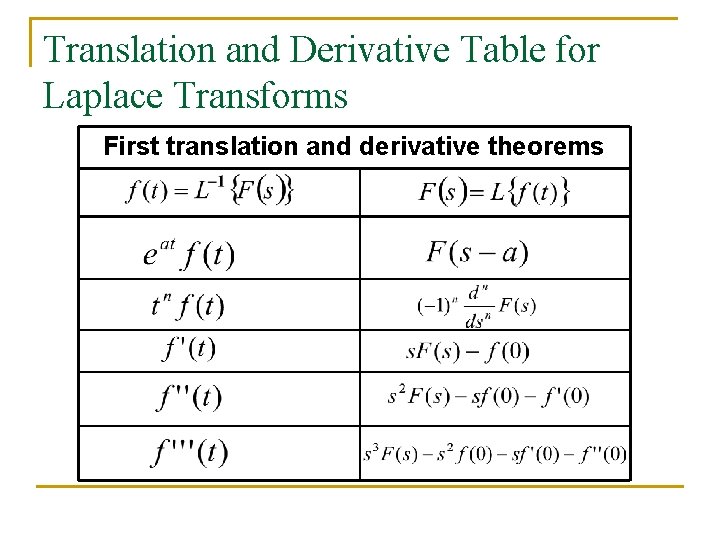
Translation and Derivative Table for Laplace Transforms First translation and derivative theorems

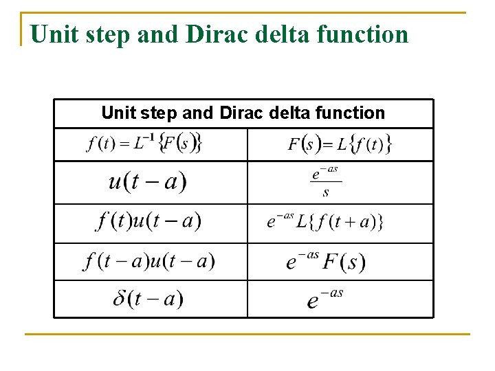
Unit step and Dirac delta function

Convolution theorem

LAPLACE TRANSFORMS SOLUTION PROCESS

Solution process (1 of 8) n Any nonhomogeneous linear differential equation with constant coefficients can be solved with the following procedure, which reduces the solution to algebra 4. Laplace transforms

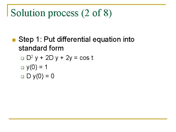
Solution process (2 of 8) n Step 1: Put differential equation into standard form q q q D 2 y + 2 D y + 2 y = cos t y(0) = 1 D y(0) = 0

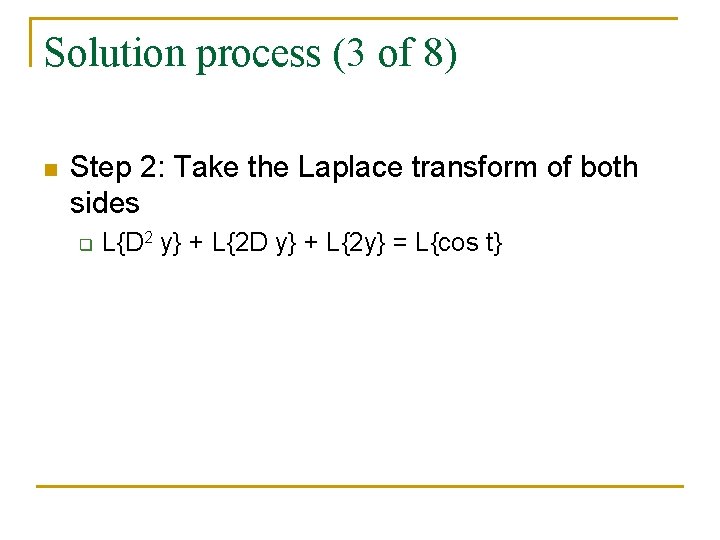
Solution process (3 of 8) n Step 2: Take the Laplace transform of both sides q L{D 2 y} + L{2 D y} + L{2 y} = L{cos t}

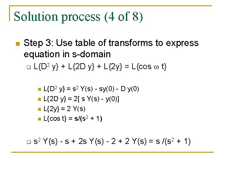
Solution process (4 of 8) n Step 3: Use table of transforms to express equation in s-domain q L{D 2 y} + L{2 D y} + L{2 y} = L{cos t} n n q L{D 2 y} = s 2 Y(s) - sy(0) - D y(0) L{2 D y} = 2[ s Y(s) - y(0)] L{2 y} = 2 Y(s) L{cos t} = s/(s 2 + 1) s 2 Y(s) - s + 2 s Y(s) - 2 + 2 Y(s) = s /(s 2 + 1)

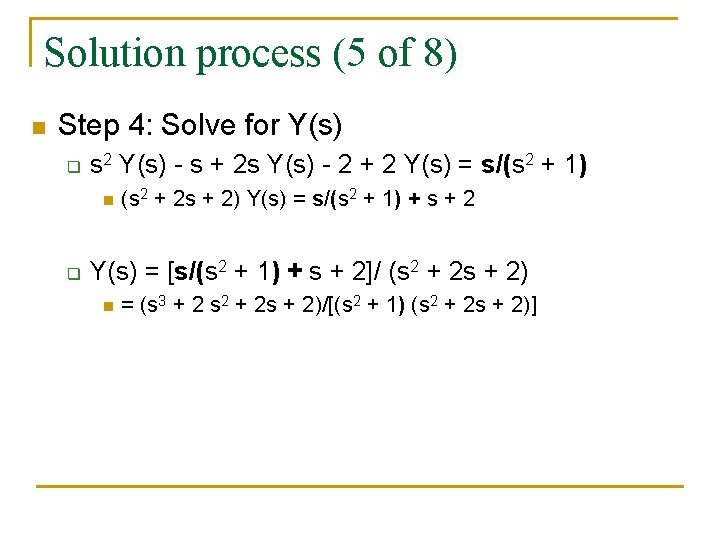
Solution process (5 of 8) n Step 4: Solve for Y(s) q s 2 Y(s) - s + 2 s Y(s) - 2 + 2 Y(s) = s/(s 2 + 1) n q (s 2 + 2 s + 2) Y(s) = s/(s 2 + 1) + s + 2 Y(s) = [s/(s 2 + 1) + s + 2]/ (s 2 + 2 s + 2) n = (s 3 + 2 s 2 + 2 s + 2)/[(s 2 + 1) (s 2 + 2 s + 2)]

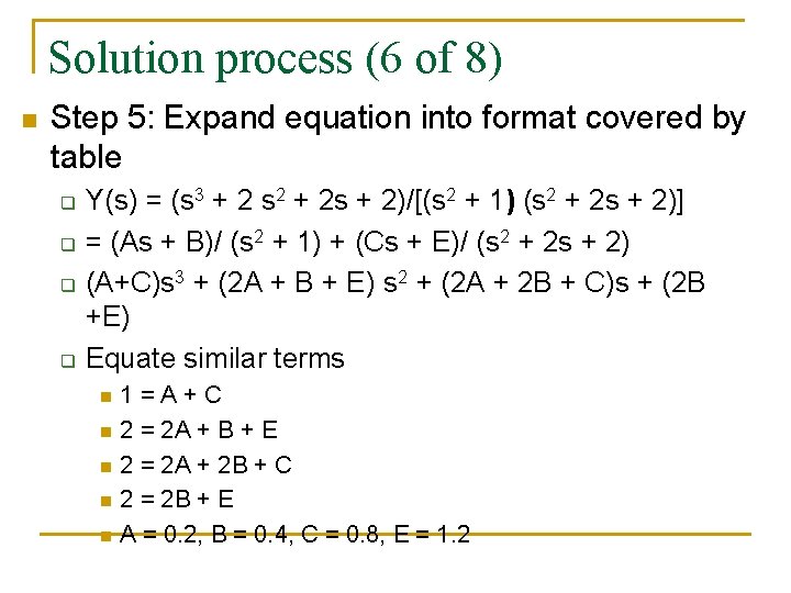
Solution process (6 of 8) n Step 5: Expand equation into format covered by table q q Y(s) = (s 3 + 2 s 2 + 2 s + 2)/[(s 2 + 1) (s 2 + 2 s + 2)] = (As + B)/ (s 2 + 1) + (Cs + E)/ (s 2 + 2 s + 2) (A+C)s 3 + (2 A + B + E) s 2 + (2 A + 2 B + C)s + (2 B +E) Equate similar terms n n n 1=A+C 2 = 2 A + B + E 2 = 2 A + 2 B + C 2 = 2 B + E A = 0. 2, B = 0. 4, C = 0. 8, E = 1. 2

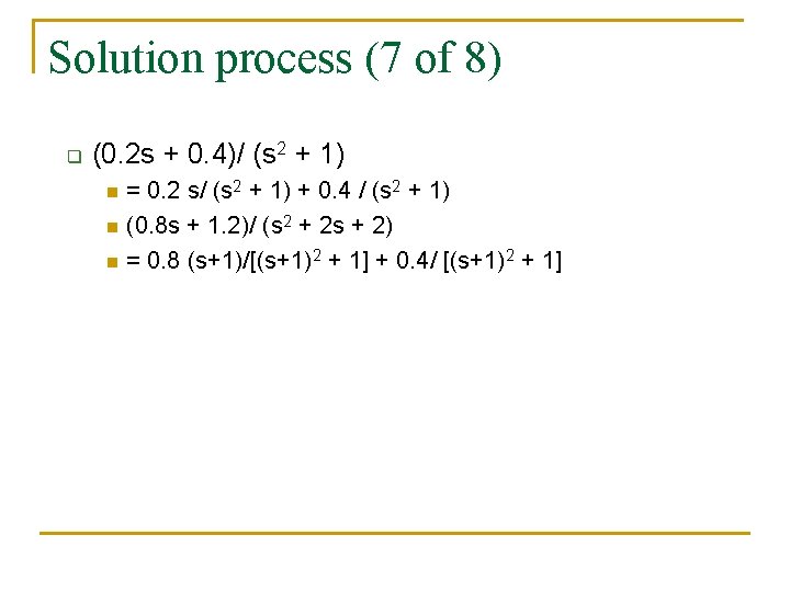
Solution process (7 of 8) q (0. 2 s + 0. 4)/ (s 2 + 1) n n n = 0. 2 s/ (s 2 + 1) + 0. 4 / (s 2 + 1) (0. 8 s + 1. 2)/ (s 2 + 2 s + 2) = 0. 8 (s+1)/[(s+1)2 + 1] + 0. 4/ [(s+1)2 + 1]

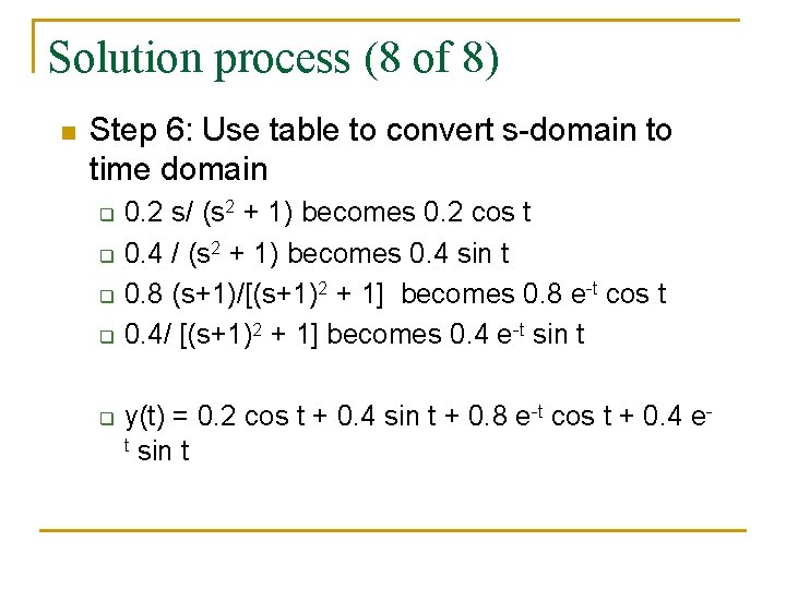
Solution process (8 of 8) n Step 6: Use table to convert s-domain to time domain q q q 0. 2 s/ (s 2 + 1) becomes 0. 2 cos t 0. 4 / (s 2 + 1) becomes 0. 4 sin t 0. 8 (s+1)/[(s+1)2 + 1] becomes 0. 8 e-t cos t 0. 4/ [(s+1)2 + 1] becomes 0. 4 e-t sin t y(t) = 0. 2 cos t + 0. 4 sin t + 0. 8 e-t cos t + 0. 4 et sin t

LAPLACE TRANSFORMS PARTIAL FRACTION EXPANSION

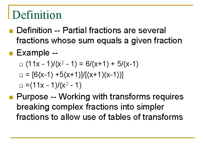
Definition n n Definition -- Partial fractions are several fractions whose sum equals a given fraction Example -q q q n (11 x - 1)/(x 2 - 1) = 6/(x+1) + 5/(x-1) = [6(x-1) +5(x+1)]/[(x+1)(x-1))] =(11 x - 1)/(x 2 - 1) Purpose -- Working with transforms requires breaking complex fractions into simpler fractions to allow use of tables of transforms

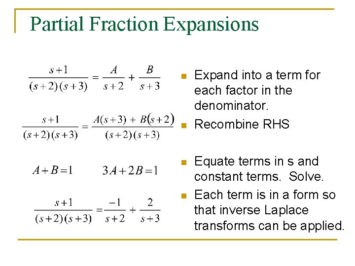
Partial Fraction Expansions n n Expand into a term for each factor in the denominator. Recombine RHS Equate terms in s and constant terms. Solve. Each term is in a form so that inverse Laplace transforms can be applied.

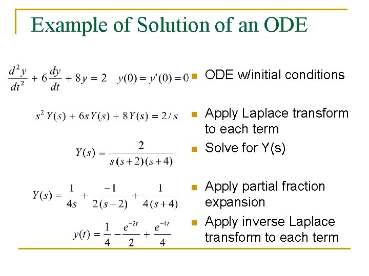
Example of Solution of an ODE w/initial conditions n Apply Laplace transform to each term Solve for Y(s) n n n Apply partial fraction expansion Apply inverse Laplace transform to each term

Different terms of 1 st degree n n To separate a fraction into partial fractions when its denominator can be divided into different terms of first degree, assume an unknown numerator for each fraction Example -q q q (11 x-1)/(X 2 - 1) = A/(x+1) + B/(x-1) = [A(x-1) +B(x+1)]/[(x+1)(x-1))] A+B=11 -A+B=-1 A=6, B=5

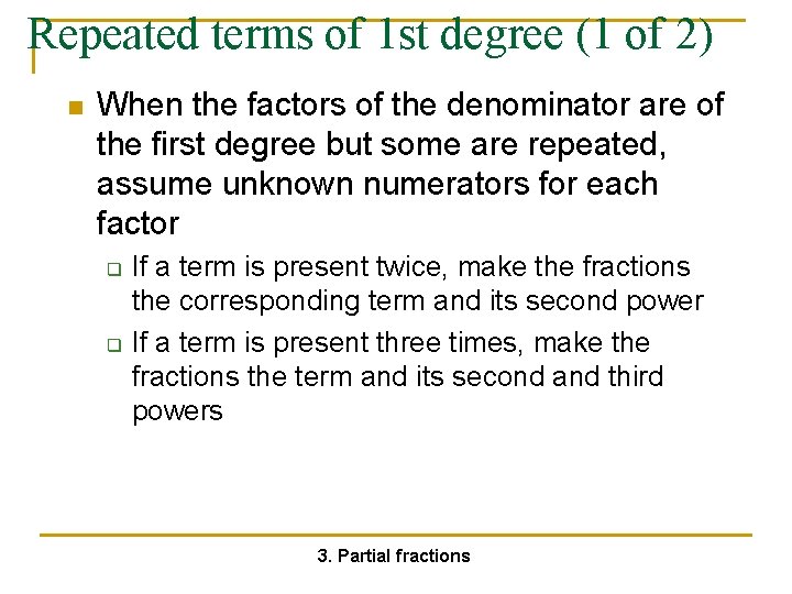
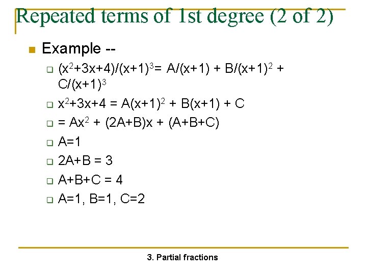
Repeated terms of 1 st degree (1 of 2) n When the factors of the denominator are of the first degree but some are repeated, assume unknown numerators for each factor q q If a term is present twice, make the fractions the corresponding term and its second power If a term is present three times, make the fractions the term and its second and third powers 3. Partial fractions

Repeated terms of 1 st degree (2 of 2) n Example -q q q q (x 2+3 x+4)/(x+1)3= A/(x+1) + B/(x+1)2 + C/(x+1)3 x 2+3 x+4 = A(x+1)2 + B(x+1) + C = Ax 2 + (2 A+B)x + (A+B+C) A=1 2 A+B = 3 A+B+C = 4 A=1, B=1, C=2 3. Partial fractions

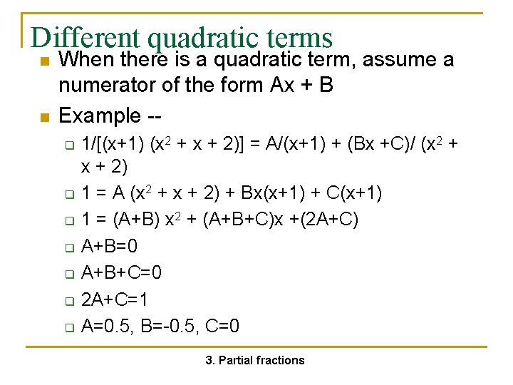
Different quadratic terms n n When there is a quadratic term, assume a numerator of the form Ax + B Example -q q q q 1/[(x+1) (x 2 + x + 2)] = A/(x+1) + (Bx +C)/ (x 2 + x + 2) 1 = A (x 2 + x + 2) + Bx(x+1) + C(x+1) 1 = (A+B) x 2 + (A+B+C)x +(2 A+C) A+B=0 A+B+C=0 2 A+C=1 A=0. 5, B=-0. 5, C=0 3. Partial fractions

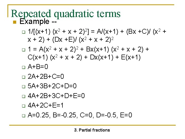
Repeated quadratic terms n Example -q q q q 1/[(x+1) (x 2 + x + 2)2] = A/(x+1) + (Bx +C)/ (x 2 + x + 2) + (Dx +E)/ (x 2 + x + 2)2 1 = A(x 2 + x + 2)2 + Bx(x+1) (x 2 + x + 2) + C(x+1) (x 2 + x + 2) + Dx(x+1) + E(x+1) A+B=0 2 A+2 B+C=0 5 A+3 B+2 C+D=0 4 A+2 B+3 C+D+E=0 4 A+2 C+E=1 A=0. 25, B=-0. 25, C=0, D=-0. 5, E=0 3. Partial fractions

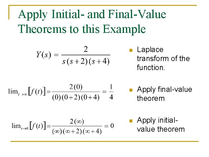
Apply Initial- and Final-Value Theorems to this Example n Laplace transform of the function. n Apply final-value theorem n Apply initialvalue theorem

LAPLACE TRANSFORMS TRANSFER FUNCTIONS

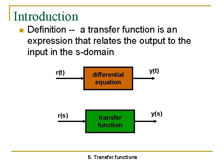
Introduction n Definition -- a transfer function is an expression that relates the output to the input in the s-domain r(t) r(s) differential equation transfer function 5. Transfer functions y(t) y(s)

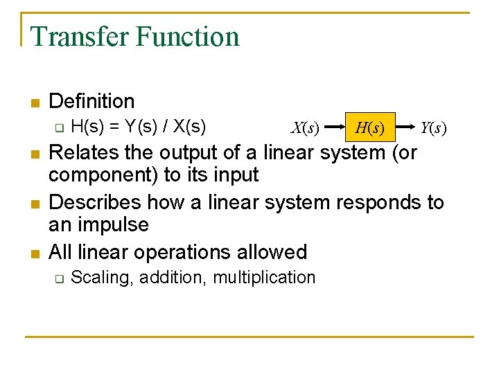
Transfer Function n Definition q n n n H(s) = Y(s) / X(s) H(s) Y(s) Relates the output of a linear system (or component) to its input Describes how a linear system responds to an impulse All linear operations allowed q Scaling, addition, multiplication

Block Diagrams n n n Pictorially expresses flows and relationships between elements in system Blocks may recursively be systems Rules q q n Cascaded (non-loading) elements: convolution Summation and difference elements Can simplify

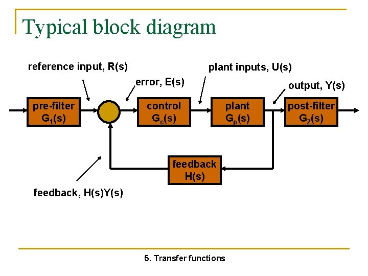
Typical block diagram reference input, R(s) plant inputs, U(s) error, E(s) pre-filter G 1(s) control Gc(s) output, Y(s) plant Gp(s) feedback H(s) feedback, H(s)Y(s) 5. Transfer functions post-filter G 2(s)

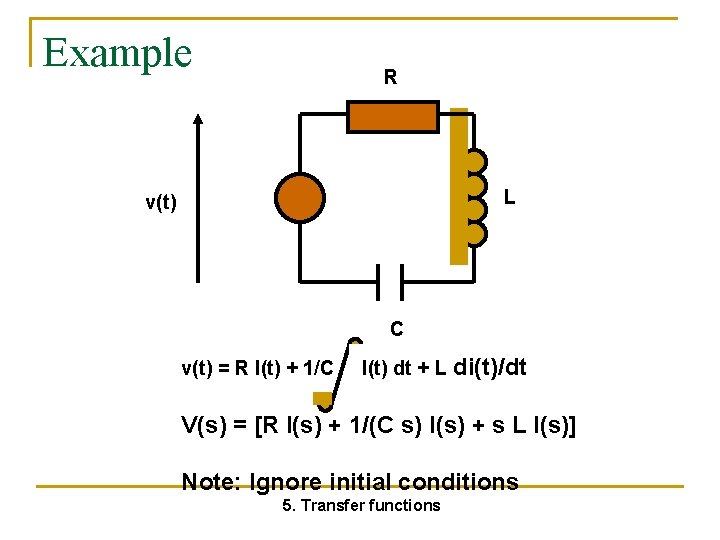
Example R L v(t) C v(t) = R I(t) + 1/C I(t) dt + L di(t)/dt V(s) = [R I(s) + 1/(C s) I(s) + s L I(s)] Note: Ignore initial conditions 5. Transfer functions

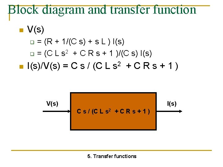
Block diagram and transfer function n V(s) q q n = (R + 1/(C s) + s L ) I(s) = (C L s 2 + C R s + 1 )/(C s) I(s)/V(s) = C s / (C L s 2 + C R s + 1 ) V(s) I(s) C s / (C L s 2 + C R s + 1 ) 5. Transfer functions

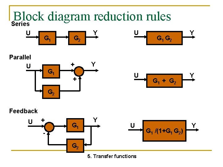
Block diagram reduction rules Series U G 1 Parallel U G 2 + G 1 Y U G 1 G 2 Y Y U + G 1 + G 2 Y G 2 Feedback U + - G 1 Y U G 2 5. Transfer functions G 1 /(1+G 1 G 2) Y

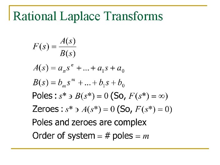
Rational Laplace Transforms

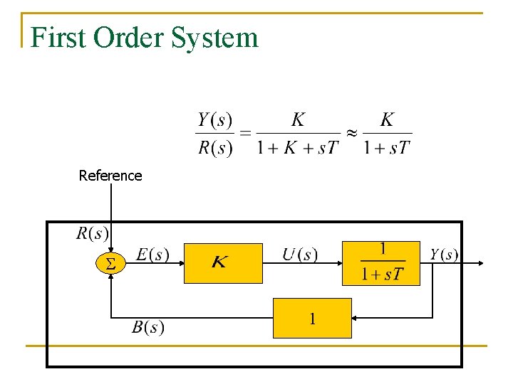
First Order System Reference S 1

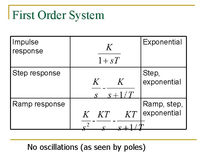
First Order System Impulse response Exponential Step response Step, exponential Ramp response Ramp, step, exponential No oscillations (as seen by poles)

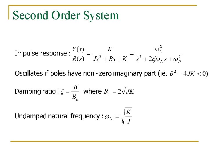
Second Order System

Second Order System: Parameters

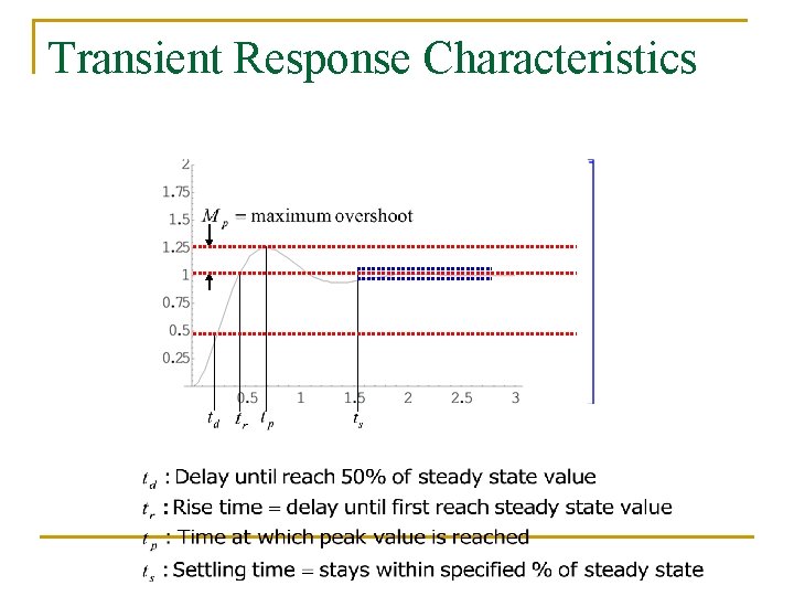
Transient Response Characteristics

Transient Response n n Estimates the shape of the curve based on the foregoing points on the x and y axis Typically applied to the following inputs q q Impulse Step Ramp Quadratic (Parabola)

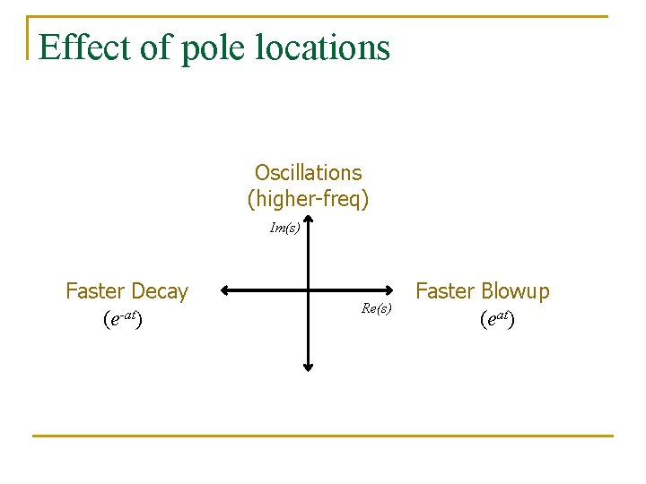
Effect of pole locations Oscillations (higher-freq) Im(s) Faster Decay (e-at) Re(s) Faster Blowup (eat)

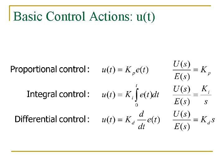
Basic Control Actions: u(t)

Effect of Control Actions n Proportional Action q n Integral Action q q n Adjustable gain (amplifier) Eliminates bias (steady-state error) Can cause oscillations Derivative Action (“rate control”) q q q Effective in transient periods Provides faster response (higher sensitivity) Never used alone

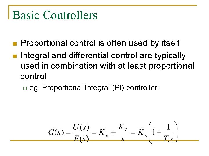
Basic Controllers n n Proportional control is often used by itself Integral and differential control are typically used in combination with at least proportional control q eg, Proportional Integral (PI) controller:

Summary of Basic Control n n Proportional control q Multiply e(t) by a constant PI control q Multiply e(t) and its integral by separate constants q Avoids bias for step PD control q Multiply e(t) and its derivative by separate constants q Adjust more rapidly to changes PID control q Multiply e(t), its derivative and its integral by separate constants q Reduce bias and react quickly

Root-locus Analysis n n Based on characteristic eqn of closed-loop transfer function Plot location of roots of this eqn q q n Multiple parameters are ok q q n Same as poles of closed-loop transfer function Parameter (gain) varied from 0 to Vary one-by-one Plot a root “contour” (usually for 2 -3 params) Quickly get approximate results q Range of parameters that gives desired response

LAPLACE TRANSFORMS LAPLACE APPLICATIONS

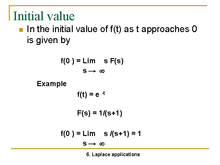
Initial value n In the initial value of f(t) as t approaches 0 is given by f(0 ) = Lim s F(s) s Example f(t) = e -t F(s) = 1/(s+1) f(0 ) = Lim s /(s+1) = 1 s 6. Laplace applications

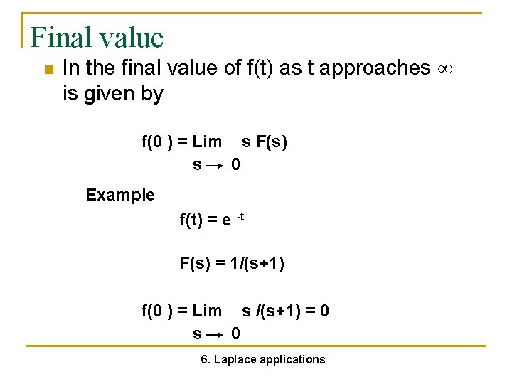
Final value n In the final value of f(t) as t approaches is given by f(0 ) = Lim s F(s) s 0 Example f(t) = e -t F(s) = 1/(s+1) f(0 ) = Lim s /(s+1) = 0 s 0 6. Laplace applications

Apply Initial- and Final-Value Theorems to this Example n Laplace transform of the function. n Apply final-value theorem n Apply initialvalue theorem

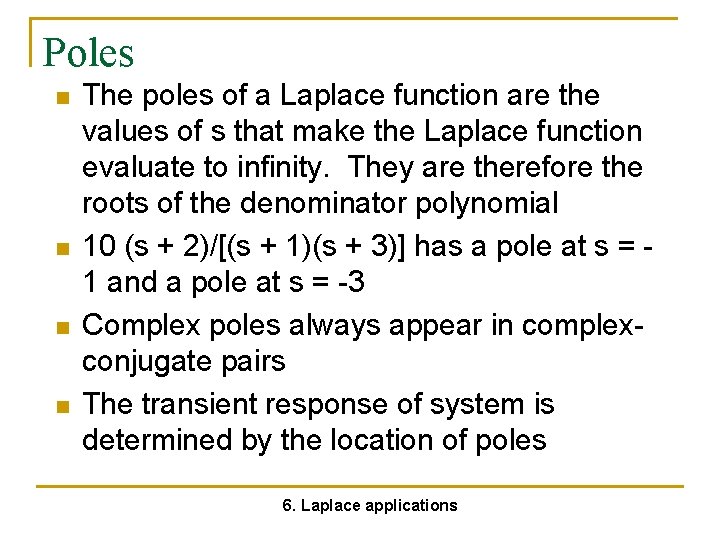
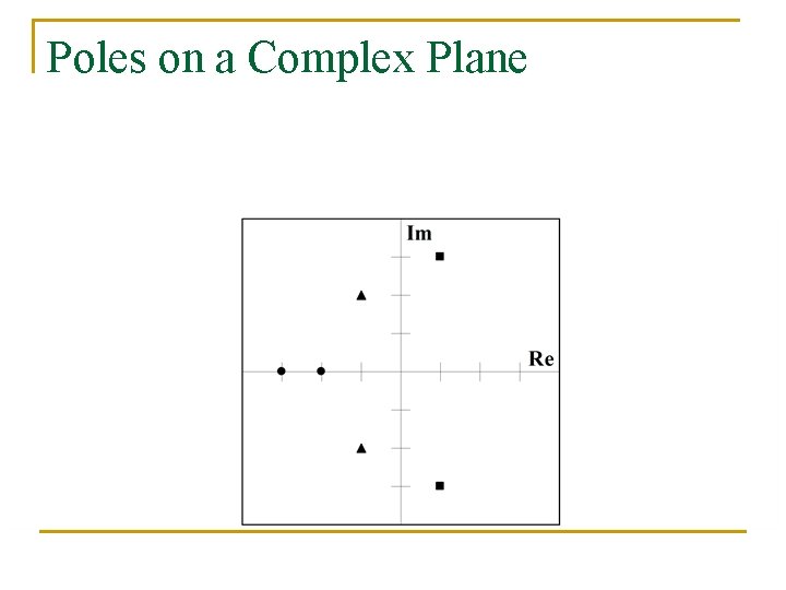
Poles n n The poles of a Laplace function are the values of s that make the Laplace function evaluate to infinity. They are therefore the roots of the denominator polynomial 10 (s + 2)/[(s + 1)(s + 3)] has a pole at s = 1 and a pole at s = -3 Complex poles always appear in complexconjugate pairs The transient response of system is determined by the location of poles 6. Laplace applications

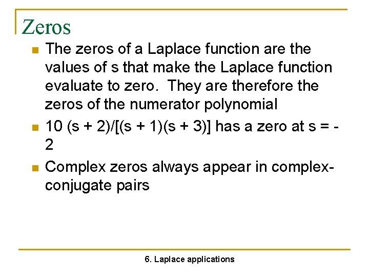
Zeros n n n The zeros of a Laplace function are the values of s that make the Laplace function evaluate to zero. They are therefore the zeros of the numerator polynomial 10 (s + 2)/[(s + 1)(s + 3)] has a zero at s = 2 Complex zeros always appear in complexconjugate pairs 6. Laplace applications

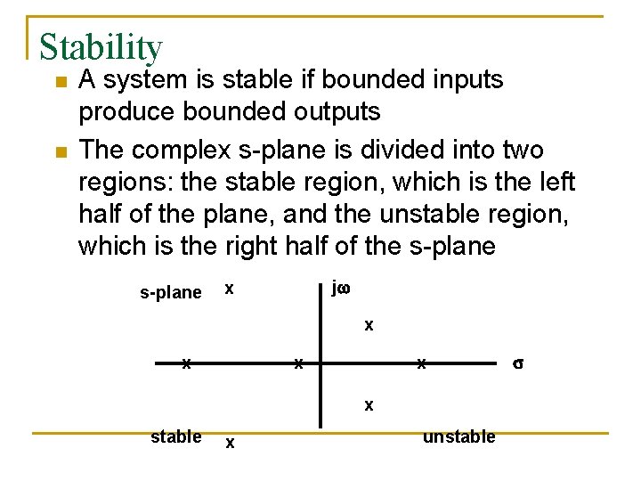
Stability n n A system is stable if bounded inputs produce bounded outputs The complex s-plane is divided into two regions: the stable region, which is the left half of the plane, and the unstable region, which is the right half of the s-plane j x x x stable x unstable

LAPLACE TRANSFORMS FREQUENCY RESPONSE

Introduction n Many problems can be thought of in the time domain, and solutions can be developed accordingly. Other problems are more easily thought of in the frequency domain. A technique for thinking in the frequency domain is to express the system in terms of a frequency response 7. Frequency response

Definition n n The response of the system to a sinusoidal signal. The output of the system at each frequency is the result of driving the system with a sinusoid of unit amplitude at that frequency. The frequency response has both amplitude and phase 7. Frequency response

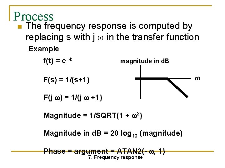
Process n The frequency response is computed by replacing s with j in the transfer function Example f(t) = e -t magnitude in d. B F(s) = 1/(s+1) F(j ) = 1/(j +1) Magnitude = 1/SQRT(1 + 2) Magnitude in d. B = 20 log 10 (magnitude) Phase = argument = ATAN 2(- , 1) 7. Frequency response

Graphical methods n n n Frequency response is a graphical method Polar plot -- difficult to construct Corner plot -- easy to construct 7. Frequency response

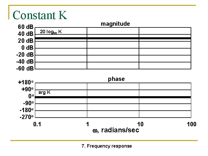
Constant K 60 d. B 40 d. B 20 d. B -20 d. B -40 d. B -60 d. B magnitude 20 log 10 K +180 o +90 o arg K 0 o -90 o -180 o -270 o 0. 1 phase 1 10 , radians/sec 7. Frequency response 100

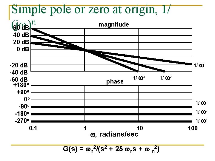
Simple pole or zero at origin, 1/ n magnitude (j ) 60 d. B 40 d. B 20 d. B -20 d. B -40 d. B -60 d. B +180 o +90 o 0 o -90 o -180 o -270 o 0. 1 1/ phase 1/ 3 1/ 2 1/ 3 1 10 , radians/sec G(s) = n 2/(s 2 + 2 ns + n 2) 100

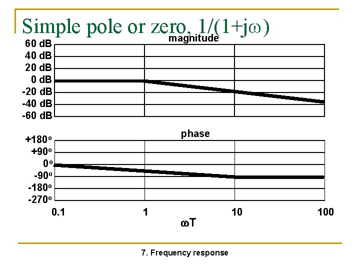
Simple pole or zero, 1/(1+j ) magnitude 60 d. B 40 d. B 20 d. B -20 d. B -40 d. B -60 d. B +180 o +90 o 0 o -90 o -180 o -270 o 0. 1 phase 1 T 7. Frequency response 10 100

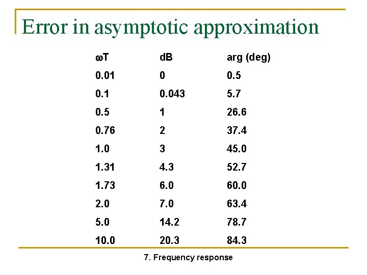
Error in asymptotic approximation T d. B arg (deg) 0. 01 0 0. 5 0. 1 0. 043 5. 7 0. 5 1 26. 6 0. 76 2 37. 4 1. 0 3 45. 0 1. 31 4. 3 52. 7 1. 73 6. 0 60. 0 2. 0 7. 0 63. 4 5. 0 14. 2 78. 7 10. 0 20. 3 84. 3 7. Frequency response

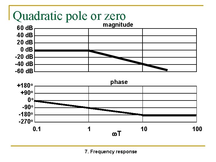
Quadratic pole or zero magnitude 60 d. B 40 d. B 20 d. B -20 d. B -40 d. B -60 d. B +180 o +90 o 0 o -90 o -180 o -270 o 0. 1 phase 1 T 7. Frequency response 10 100

Transfer Functions n n Defined as G(s) = Y(s)/U(s) Represents a normalized model of a process, i. e. , can be used with any input. Y(s) and U(s) are both written in deviation variable form. The form of the transfer function indicates the dynamic behavior of the process.

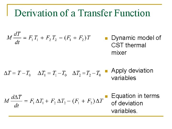
Derivation of a Transfer Function n Dynamic model of CST thermal mixer n Apply deviation variables n Equation in terms of deviation variables.

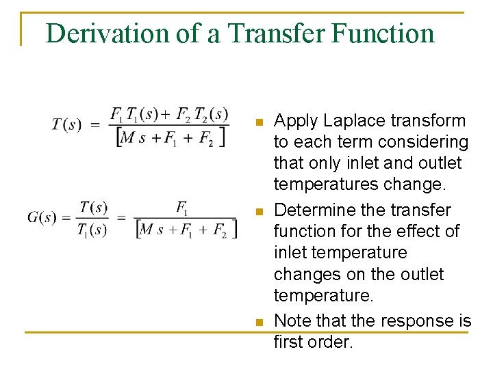
Derivation of a Transfer Function n Apply Laplace transform to each term considering that only inlet and outlet temperatures change. Determine the transfer function for the effect of inlet temperature changes on the outlet temperature. Note that the response is first order.

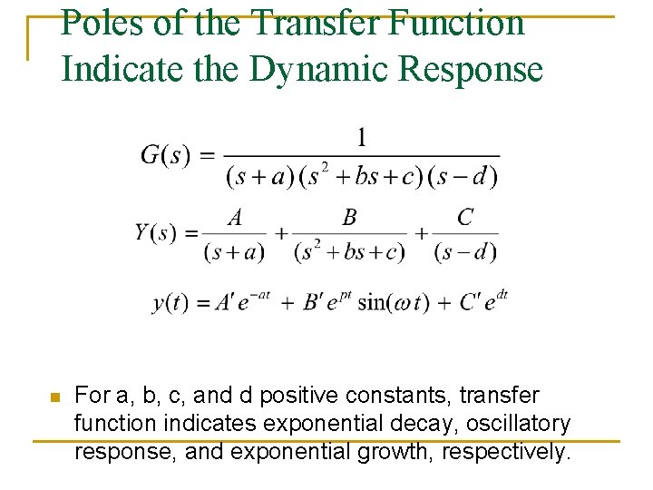
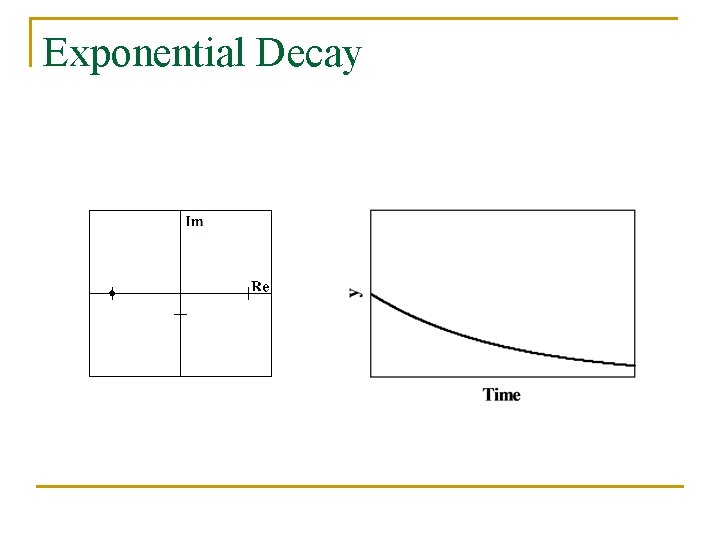
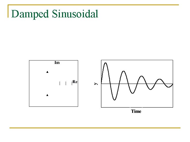
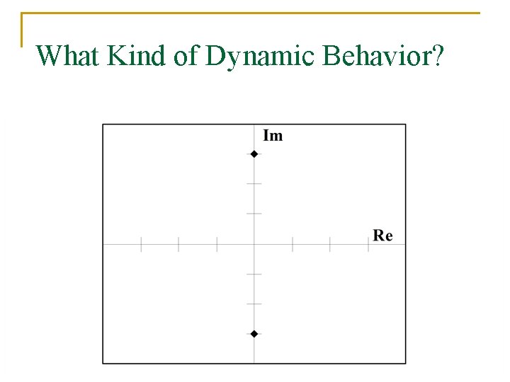
Poles of the Transfer Function Indicate the Dynamic Response n For a, b, c, and d positive constants, transfer function indicates exponential decay, oscillatory response, and exponential growth, respectively.

Poles on a Complex Plane

Exponential Decay

Damped Sinusoidal

Exponentially Growing Sinusoidal Behavior (Unstable)

What Kind of Dynamic Behavior?

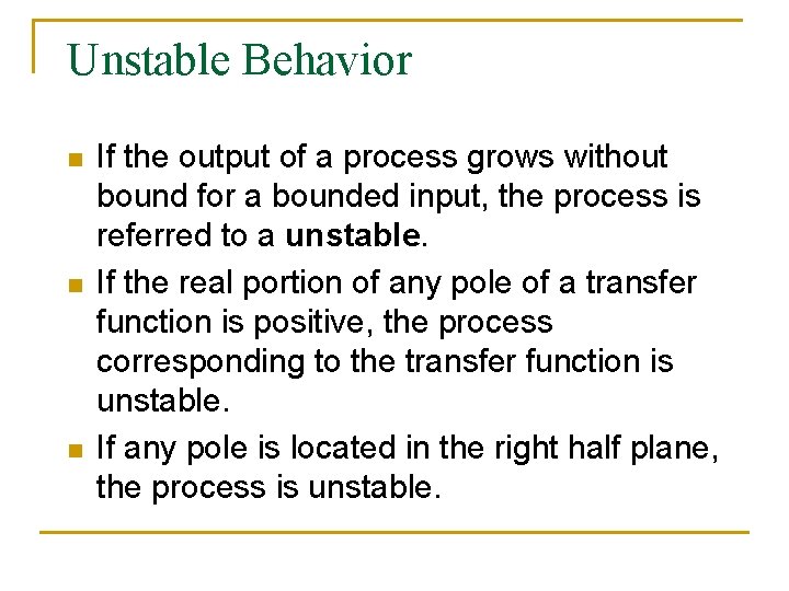
Unstable Behavior n n n If the output of a process grows without bound for a bounded input, the process is referred to a unstable. If the real portion of any pole of a transfer function is positive, the process corresponding to the transfer function is unstable. If any pole is located in the right half plane, the process is unstable.