7 2 Ordinary Differential Equations with Initial Values

7. 2 Ordinary Differential Equations with Initial Values • Many of the problems encountered in physics involve ordinary differential equations for which some initial values are specified. For example, the motion of a projectile is described by second – order differential equations that involve the position as a function of time. For these problems, we would like to find the quantity of interest (such as the position of the projectile) as a function of time. In other words, we want to propagate the relevant function forward in time starting from the given initial value. • There are several ways to attack such problems numerically, and which ones are appropriate or effective depends on the problem.

7. 2. 1 First–ORDER, ORDINARY DIFFERENTIAL EQUATIONS • We begin by considering first order ordinary differential equations of the from • With the initial condition that x(0) =x 0. In this case, the Taylor series expansion of x around t gives

• Thus, assuming a reasonably smooth function x (t) and a small interval ∆t, we can propagate x (t) to x (t +∆t) to any accuracy desired as long as we know the derivatives of x (t). • However, we often do not know the derivatives for general for values of t, and we also want to propagate for much more than an infinitesimally small interval ∆t. So we are faced with the problem of estimating derivative (s) of an unknown function as well as the need to repeat the propagation by ∆t many times. Different ways of doing this yield different approximations associated with different levels of error.

• If we are somehow given x (t i), the exact value of x at time t i = i ∆t, propagation forward with the Euler method gives • x ( ti + 1 ) ≈ x (ti) + f (x(ti), ti) ∆t (7. 2. 3) • The symbol here reminds us that right – hand side in (2. 3) is only an approximation for the exact value x (ti +1). The local order of a particular approximation is determined by the order in ∆t (or whatever the expansion parameter happens to be) to which the approximation agrees with the exact solution.

• Comparing (7. 2. 3) and (7. 2. 2) we see that the Euler method is locally a first order approximation at ti + 1, and it is easy to see that it remains so at later values t also. If we want to calculate x (b) for some fixed value of t = b, starting from t = 0, then the Euler propagation step must be repeated N = b / ∆t times. Since the error is of the order of (∆t)2 at each step, the final estimate for x (b) will have an error or order N (∆t)2 a ∆t. According to the conventional terminology, the Euler method could reduce the actual error by reducing ∆t, the error at t = b is only reduced linearly as ∆t (and the computing requirements go up linearly).

• With the Euler method, and with all other approaches, the choice of ∆t is very important. Smaller values of ∆t will give smaller errors (if one ignores the possibility of round – off error), but reducing ∆t leads to greater computational cost (i. e, more steps and a longer run time for your program). On the other hand, too large a value of ∆t can make an approximation unstable or meaningless. For example, in our nuclear decay problem, f (x , t) = – x / T where T is the decay time constant. Thus the first Euler propagation step gives

• If one takes ∆t = T, this approximation becomes x (t)=0, and even worse, if ∆t > T is taken, the Euler result for x (t) oscillates in sign. • How can we systematically improve the situation? One obvious answer is to keep to higher order in the Taylor expansion. For example, we could take an iterative approach

• Where the subscript i on the derivatives indicates evaluation at Xi and • t = ti. While this would produce an approximation that is locally of second order and globally of first order, a drawback of this approach is that the partial derivatives of f (x , t) must be evaluated. tm • Many other approaches can be constructed which yield the same order of approximation without the explicit need to evaluate the partial derivatives. In this context, it may be useful to think of the problem as the integration of d x / d t from, say, t to t + ∆t. According to the mean value theorem, there is a value tm in the interval { t, t + ∆t} such that the exact solution can be gotten while stopping at first order in ∆t

In this sense, the slope d X / d t incorporates the effects of the curvature (the second and higher order terms) present in the Taylor expansion. Of course we do not generally know tm or the slope, and thus must somehow estimate them approximately. The Euler method replaces tm by t on the right – hand side of this equation. Graphically, this corresponds to linearly extrapolating up to (t+∆t) by using a line tangent to x (t) at (see Figure 7. 2. 1).

FIGURE 7. 2. 1: Geometrical interpretation of Euler method.

• Even though the above expression resembles the Taylor expansion truncated at the first order, they are not same. By estimating tm and • d x / dt/tm intelligently, we can effectively construct approximations of higher order than the Euler method. A popular example is the Runge – Kutta methods. The most common second–order Runge – Kutta approximation is constructed by

• In other words, the slope d x / d t tm is estimated as the value f (x 1, t 1) where t 1. is the midpoint of the interval and x 1 is the Euler approximated value of x at t 1 it is easy to show that this approximation is indeed locally of second order { i. e. , agreeing with the Taylor expansion up to order(∆t)2}, and of first order globally. This means that the error in x (b) for fixed b can be reduced quadratically by reducing ∆t. • The cost of the increased accuracy of(7. 2. 7) is a large computational requirement. For each step of propagating by ∆t, we must first obtain

• (x 1, t 1) by the Euler method and then substitute the results into (7. 2. 7), so we have roughly twice the computing requirement of the Euler method. One way to put the relative computational costs in perspective is to estimate the resources required to obtain comparable accuracy by using different methods. When making such comparisons it is useful to think of the Taylor expansion in terms a dimensionless expansion parameter. By keeping the same ∆t but going to the second – order Runge – Kutta method, we may expect to improve the accuracy by a factor of about 100. On the other hand, we would have to reduce ∆t by the same factor to achieve a comparable improvement using the Euler method. Since the Runge – Kutta approach only doubles the computational the requirement while this change in the Euler approach would increase it by 100 – fold, the values of these numerical errors depend very much on the exact coefficients in our Taylor expansions, and thus on the functional from of f (x, t). in addition, anyway for smooth interpolation.

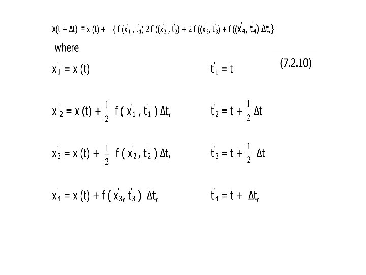
• There are many other possible second – order approximations, as there are many ways to approximate the slop d x / d ttm in (7. 2. 6) in such a way as to agree with the Taylor expansion up to second order. In general Runge – Kutta approximations, one estimates this slope by a weighted average of several terms of the from f (x 1 i, ti 1) where x 1 i (i = 1, 2, . . ) are suitably chosen values in the interval {t, t + ∆ t}, and x 1 i are obtained by some Euler or Euler – like approximation for x (x 1 i). even limiting ourselves to this type of approximation, there are infinite number of second– order choices. A popular higher order approximation is the forth – order Runge – Kutta method defined by

7. 2. 2 SECOND – ORDER, ORDINARY DIFFERENTIAL EQUATIONS • In many cases encountered in physics it is the second derivative that can be calculated. For example, if y is the position of an object, then Newton's second law tells us that the second derivative d 2 y / d t 2 is equal to the force on the object divided by the mass. Initial value problems of this kind are typically solved numerically by starting from the known initial values yo = y (to) and uo = d y / d t ( y o. to) and propagating forward in t with ti Ξ t 0 + i ∆t. we begin by converting the problem into one involving two first – order differential equations

• • • f 2 (y, t) where f 2 (y, t) is our second derivative function • To apply the Euler method we write each of these first derivatives in finite difference from, truncating the Taylor expansion at first order. Proceeding as we did in the first – order case yields • y (ti + 1) ≈ y (ti) + v (ti) ∆t v (ti +1) ≈ v (ti) + f 2 { y (ti ), ti }∆t, • where the ≈ symbols remind us again that the right – hand sides here are only approximations to the true solution. Geometrically this has same interpretation as in Figure 2. 1. The derivatives evaluated at (yi , ti) are used make linear extrapolations to obtain estimates of vi +1 and. Yi+1.

• There are many ways to deal with this instability problem. One obvious method might to be reduce ∆t and hope to achieve better accuracy. While this works to some extent, the errors still tend to accumulate and the instability eventually resurfaces. Another way is go to a higher order approximation such as the Rung – Kutta methods of second or higher order, where the errors in, e. g. , energy will be of higher order too, though they may still accumulate over many periods. • There is, however, a simple modification of the Euler method which sometimes cures the problem of error accumulation at O {(∆t)2}. We have seen that the Euler method uses yi and vi, the estimates for y and v at time step i, to calculate the estimates at the next time step i + 1. A slight change in this procedure yields the Euler – Cromer method. With this method we use yi and vi to estimate vi + 1 but then use yi and vi + 1 to estimate yi + 1.

• We could justify this in part by arguing as follows. Part of the problem with the Euler method is the one – sided approximation of the slopedx/d t tm appearing in the mean value theorem(7. 2. 6). This problem can be reduced by using a more symmetric evaluation of d y/d t and d v/dt, namely, evaluating d v/d t at t while evaluating dv/dt at t+ ∆t. In fact, careful analysis shows that for oscillatory problems this algorithm actually conserves energy over each complete oscillation at least O {(∆t)2. This makes it a better choice for problem such as simple harmonic motion than the Euler method. • However, we want to caution that while the Euler – Cromer method is preferable to the Euler algorithm for oscillatory problems, the overall accuracy of the two methods for other types of problems is usually comparable as the Euler – Cromer method for (7. 2. 11) is still a locally first approximation just like the Euler method. In particular, while the Euler – Cromer method conserves the total energy over integer periods in oscillatory problems, this is not necessarily the case in other situations.

• As an example of using a higher – order approximation to curb the problems of instability in oscillatory solutions, we again consider the simple harmonic oscillator problem, but this time use the second – order Runge – Kutta , method. The second – order Runge – Kutta equations in this case are