IME 634 Management Decision Analysis Raghu Nandan Sengupta

IME 634: Management Decision Analysis Raghu Nandan Sengupta Industrial & Management Department Indian Institute of Technology Kanpur IME 634: MDA RNSengupta, IME Dept. , IIT Kanpur, INDIA 1

Utility Analysis Consider the same type of construction project is being undertaken by more than one company, who we will consider are the investors. Now different investors (considering they are investing their money, time, energy, skill, etc. ) have different attributes and risk perception for the same project That is to say, each investor has with him/her an opportunity set. This opportunity set is specific to that person only. IME 634: MDA RNSengupta, IME Dept. , IIT Kanpur, INDIA 2

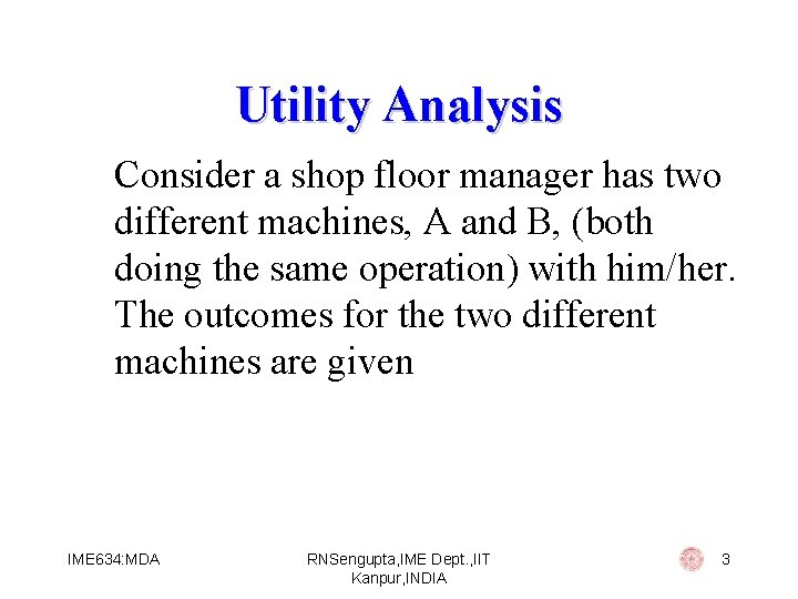
Utility Analysis Consider a shop floor manager has two different machines, A and B, (both doing the same operation) with him/her. The outcomes for the two different machines are given IME 634: MDA RNSengupta, IME Dept. , IIT Kanpur, INDIA 3

Utility Analysis A B Outcome value(i) P[i] 15 1/3 20 1/3 12 1/3 15 1/3 8 1/3 In reality what would a person do if he or she has two outcome sets in front of him/her. For A we have the expected value of outcome as 13. 33 and for B also it is 13. 33 IME 634: MDA RNSengupta, IME Dept. , IIT Kanpur, INDIA 4

Utility Analysis A B Outcome value(i) P[i] 15 ½ 20 1/3 10 ¼ 12 1/3 15 ¼ 8 1/3 Now for A we have the expected value of outcome as 13. 75 and for B it is still 13. 33. IME 634: MDA RNSengupta, IME Dept. , IIT Kanpur, INDIA 5

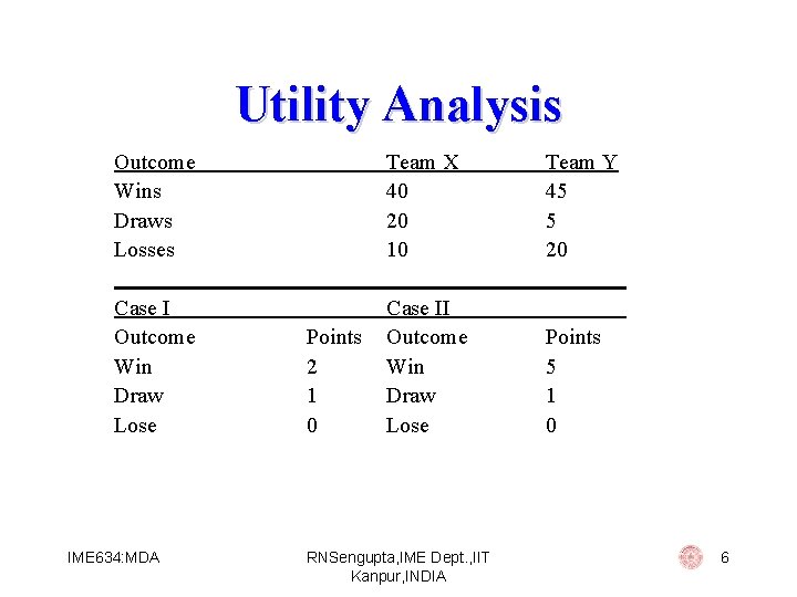
Utility Analysis Outcome Wins Draws Losses Team X 40 20 10 Team Y 45 5 20 Case I Outcome Win Draw Lose Case II Outcome Win Draw Lose Points 5 1 0 IME 634: MDA Points 2 1 0 RNSengupta, IME Dept. , IIT Kanpur, INDIA 6

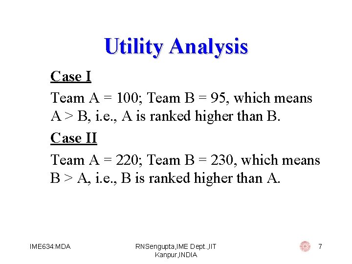
Utility Analysis Case I Team A = 100; Team B = 95, which means A > B, i. e. , A is ranked higher than B. Case II Team A = 220; Team B = 230, which means B > A, i. e. , B is ranked higher than A. IME 634: MDA RNSengupta, IME Dept. , IIT Kanpur, INDIA 7

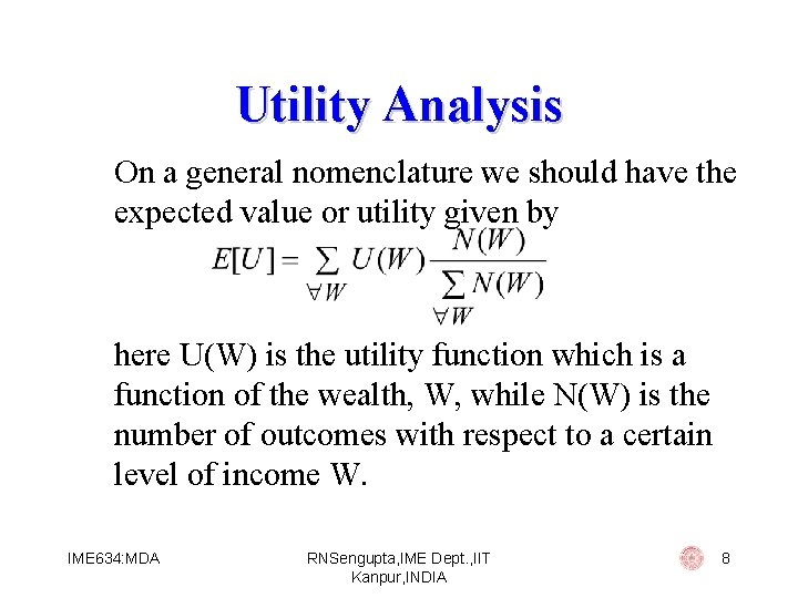
Utility Analysis On a general nomenclature we should have the expected value or utility given by here U(W) is the utility function which is a function of the wealth, W, while N(W) is the number of outcomes with respect to a certain level of income W. IME 634: MDA RNSengupta, IME Dept. , IIT Kanpur, INDIA 8

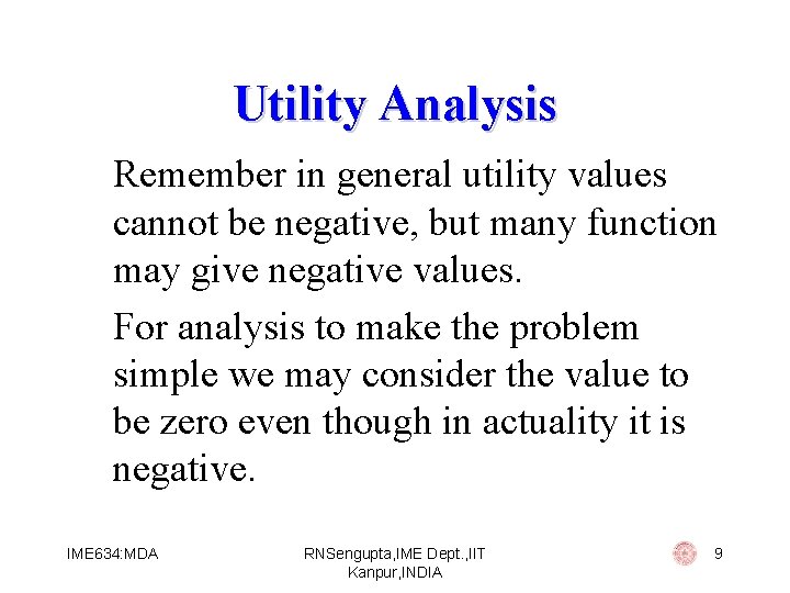
Utility Analysis Remember in general utility values cannot be negative, but many function may give negative values. For analysis to make the problem simple we may consider the value to be zero even though in actuality it is negative. IME 634: MDA RNSengupta, IME Dept. , IIT Kanpur, INDIA 9

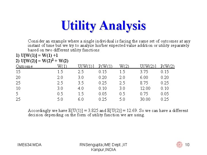
Utility Analysis Consider an example where a single individual is facing the same set of outcomes at any instant of time but we try to analyze his/her expected value addition or utility separately based on two different utility functions 1) U[W(1)] = W(1) +1 2) U[W(2)] = W(2)2 + W(2) Outcome W(1) U[W(1)] P(W(1) W(2) U[W(2)] P(W(2) 15 1. 5 2. 5 0. 15 1. 5 3. 75 0. 15 20 2. 0 3. 0 0. 20 2. 0 6. 00 0. 20 25 2. 5 3. 5 0. 25 2. 5 8. 75 0. 25 10 3. 0 4. 0 0. 10 3. 0 12. 00 0. 10 5 0. 5 1. 5 0. 05 0. 75 0. 05 25 5. 0 6. 0 0. 25 5. 0 30. 00 0. 25 Accordingly we have E[U(1)] = 3. 825 and E[U(2)] = 12. 69. So we can have a different decision depending on the form of utility function we are using. IME 634: MDA RNSengupta, IME Dept. , IIT Kanpur, INDIA 10

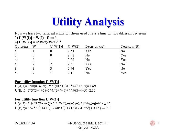
Utility Analysis Now we have two different utility functions used one at a time for two different decisions 1) U[W(1)] = W(1) - 5 and 2) U[W(2)] = 2*W(2)-W(2)1. 25 Outcome W U[W(1)] U[W(2)] Decision (A) Decision (B) 8 4 0 2. 34 Yes No 3 5 0 2. 52 No Yes 4 6 1 2. 60 No Yes 6 7 2 2. 61 Yes No 9 8 3 2. 54 Yes No 5 9 4 2. 41 No Yes For utility function U[W(1)] U(A, 1)=0*8/(8+6+9)+2*6/(8+6+9)+3*9/(8+6+9)=1. 69 U(B, 1)=0*3/(3+4+5)+1*4/(3+4+5)+4*5/(3+4+5)=2. 00 For utility function U[W(2)] U(A, 2)=2. 34*8/(8+6+9)+2. 61*6/(8+6+9)+2. 54*9/(8+6+9) 2. 50 U(B, 2)=2. 52*3/(3+4+5)+2. 60*4/(3+4+5)+2. 41*5/(3+4+5) 2. 50 IME 634: MDA RNSengupta, IME Dept. , IIT Kanpur, INDIA 11

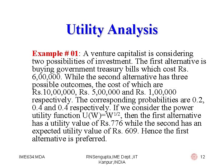
Utility Analysis Example # 01: A venture capitalist is considering two possibilities of investment. The first alternative is buying government treasury bills which cost Rs. 6, 000. While the second alternative has three possible outcomes, the cost of which are Rs. 10, 000, Rs. 5, 000 and Rs. 1, 000 respectively. The corresponding probabilities are 0. 2, 0. 4 and 0. 4 respectively. If we consider the power utility function U(W)=W 1/2, then the first alternative has a utility value of Rs. 776 while the second has an expected utility value of Rs. 609. Hence the first alternative is preferred. IME 634: MDA RNSengupta, IME Dept. , IIT Kanpur, INDIA 12

Utility Analysis Would the above problem give a different answer if we used an utility function of the form U(W) = W 1/2 + c (where c is a positive o a negative constant)? IME 634: MDA RNSengupta, IME Dept. , IIT Kanpur, INDIA 13

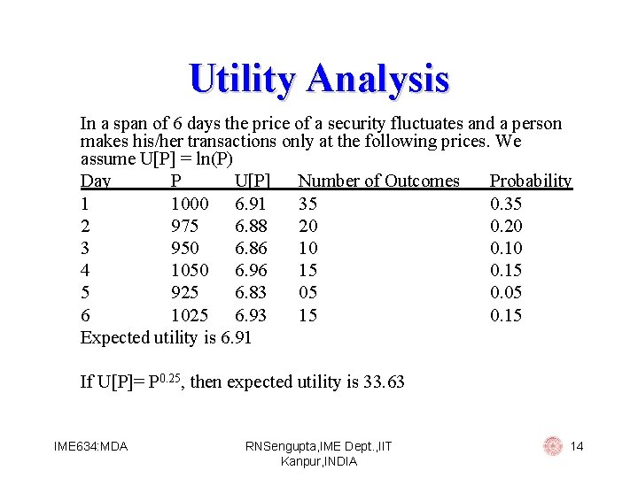
Utility Analysis In a span of 6 days the price of a security fluctuates and a person makes his/her transactions only at the following prices. We assume U[P] = ln(P) Day P U[P] Number of Outcomes Probability 1 1000 6. 91 35 0. 35 2 975 6. 88 20 0. 20 3 950 6. 86 10 0. 10 4 1050 6. 96 15 0. 15 5 925 6. 83 05 0. 05 6 1025 6. 93 15 0. 15 Expected utility is 6. 91 If U[P]= P 0. 25, then expected utility is 33. 63 IME 634: MDA RNSengupta, IME Dept. , IIT Kanpur, INDIA 14

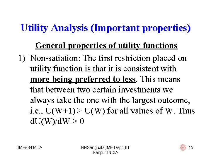
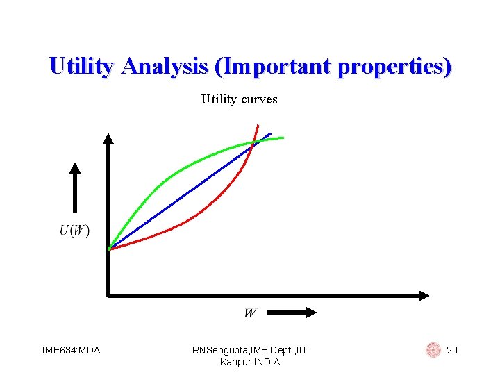
Utility Analysis (Important properties) General properties of utility functions 1) Non-satiation: The first restriction placed on utility function is that it is consistent with more being preferred to less. This means that between two certain investments we always take the one with the largest outcome, i. e. , U(W+1) > U(W) for all values of W. Thus d. U(W)/d. W > 0 IME 634: MDA RNSengupta, IME Dept. , IIT Kanpur, INDIA 15

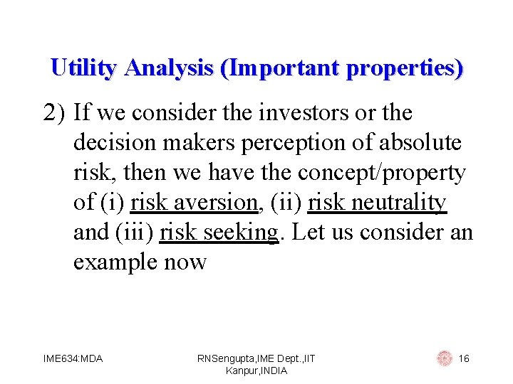
Utility Analysis (Important properties) 2) If we consider the investors or the decision makers perception of absolute risk, then we have the concept/property of (i) risk aversion, (ii) risk neutrality and (iii) risk seeking. Let us consider an example now IME 634: MDA RNSengupta, IME Dept. , IIT Kanpur, INDIA 16

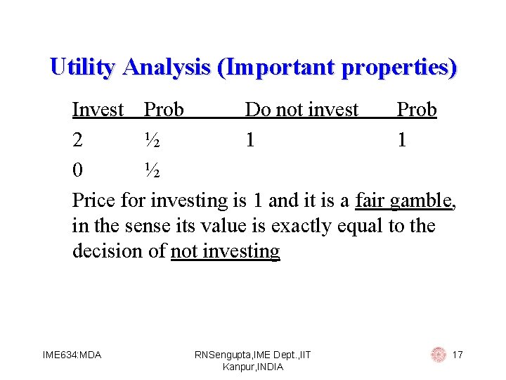
Utility Analysis (Important properties) Invest Prob Do not invest Prob 2 ½ 1 1 0 ½ Price for investing is 1 and it is a fair gamble, in the sense its value is exactly equal to the decision of not investing IME 634: MDA RNSengupta, IME Dept. , IIT Kanpur, INDIA 17

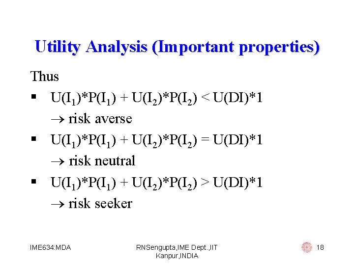
Utility Analysis (Important properties) Thus § U(I 1)*P(I 1) + U(I 2)*P(I 2) < U(DI)*1 risk averse § U(I 1)*P(I 1) + U(I 2)*P(I 2) = U(DI)*1 risk neutral § U(I 1)*P(I 1) + U(I 2)*P(I 2) > U(DI)*1 risk seeker IME 634: MDA RNSengupta, IME Dept. , IIT Kanpur, INDIA 18

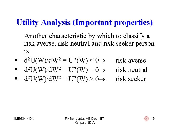
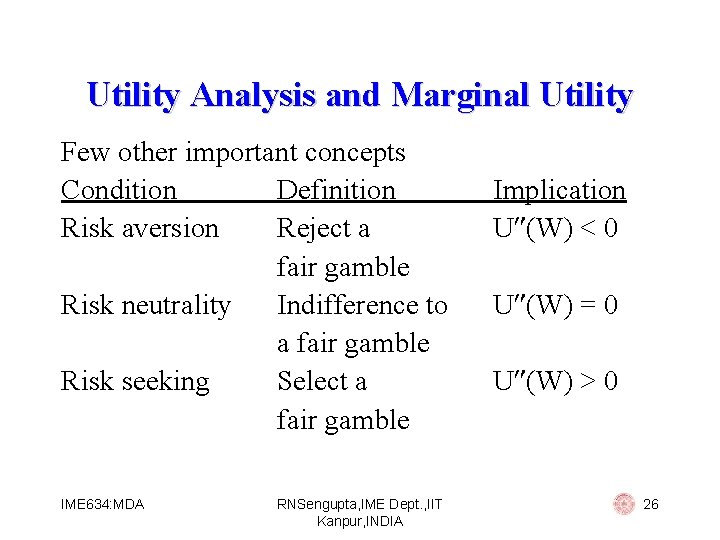
Utility Analysis (Important properties) Another characteristic by which to classify a risk averse, risk neutral and risk seeker person is § d 2 U(W)/d. W 2 = U (W) < 0 risk averse § d 2 U(W)/d. W 2 = U (W) = 0 risk neutral § d 2 U(W)/d. W 2 = U (W) > 0 risk seeker IME 634: MDA RNSengupta, IME Dept. , IIT Kanpur, INDIA 19

Utility Analysis (Important properties) Utility curves IME 634: MDA RNSengupta, IME Dept. , IIT Kanpur, INDIA 20

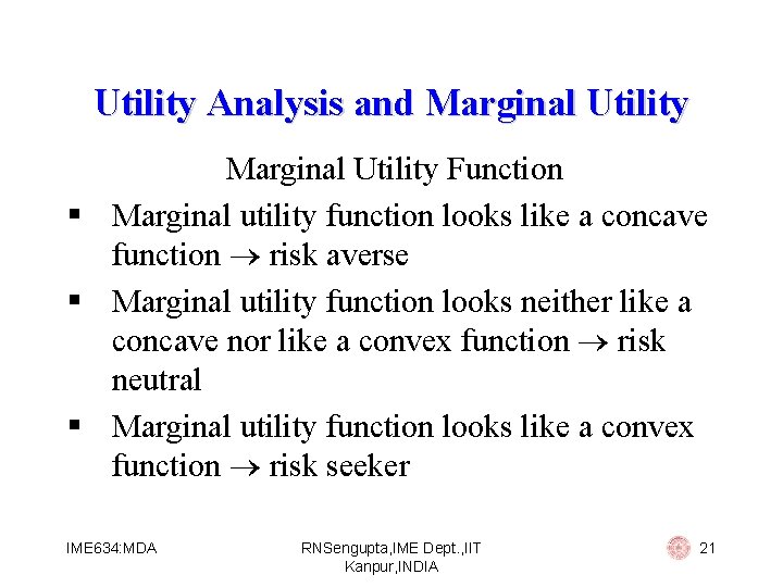
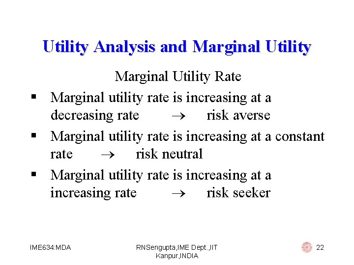
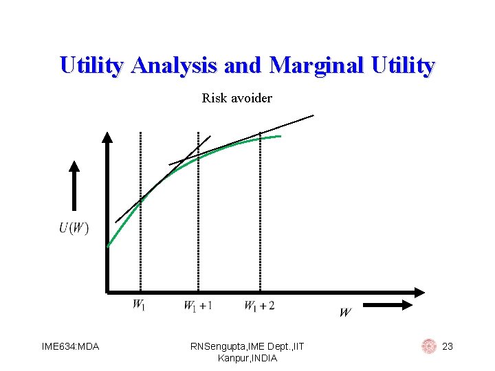
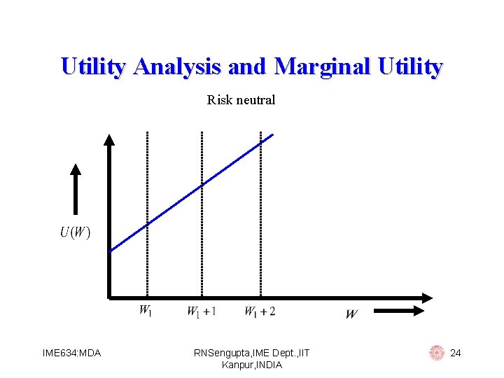
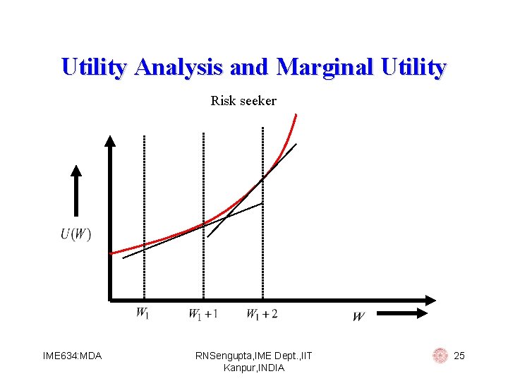
Utility Analysis and Marginal Utility Function § Marginal utility function looks like a concave function risk averse § Marginal utility function looks neither like a concave nor like a convex function risk neutral § Marginal utility function looks like a convex function risk seeker IME 634: MDA RNSengupta, IME Dept. , IIT Kanpur, INDIA 21

Utility Analysis and Marginal Utility Rate § Marginal utility rate is increasing at a decreasing rate risk averse § Marginal utility rate is increasing at a constant rate risk neutral § Marginal utility rate is increasing at a increasing rate risk seeker IME 634: MDA RNSengupta, IME Dept. , IIT Kanpur, INDIA 22

Utility Analysis and Marginal Utility Risk avoider IME 634: MDA RNSengupta, IME Dept. , IIT Kanpur, INDIA 23

Utility Analysis and Marginal Utility Risk neutral IME 634: MDA RNSengupta, IME Dept. , IIT Kanpur, INDIA 24

Utility Analysis and Marginal Utility Risk seeker IME 634: MDA RNSengupta, IME Dept. , IIT Kanpur, INDIA 25

Utility Analysis and Marginal Utility Few other important concepts Condition Definition Risk aversion Reject a fair gamble Risk neutrality Indifference to a fair gamble Risk seeking Select a fair gamble IME 634: MDA RNSengupta, IME Dept. , IIT Kanpur, INDIA Implication U (W) < 0 U (W) = 0 U (W) > 0 26

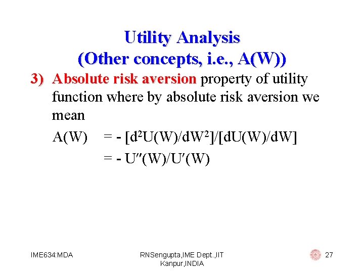
Utility Analysis (Other concepts, i. e. , A(W)) 3) Absolute risk aversion property of utility function where by absolute risk aversion we mean A(W) = - [d 2 U(W)/d. W 2]/[d. U(W)/d. W] = - U (W)/U (W) IME 634: MDA RNSengupta, IME Dept. , IIT Kanpur, INDIA 27

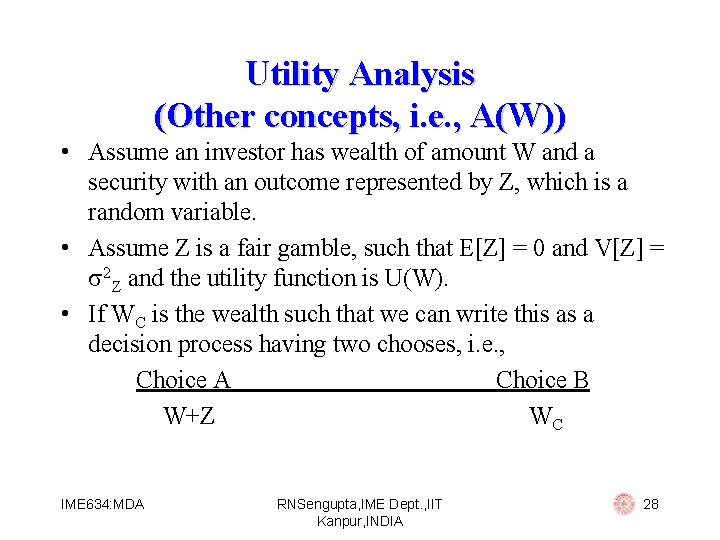
Utility Analysis (Other concepts, i. e. , A(W)) • Assume an investor has wealth of amount W and a security with an outcome represented by Z, which is a random variable. • Assume Z is a fair gamble, such that E[Z] = 0 and V[Z] = 2 Z and the utility function is U(W). • If WC is the wealth such that we can write this as a decision process having two chooses, i. e. , Choice A Choice B W+Z WC IME 634: MDA RNSengupta, IME Dept. , IIT Kanpur, INDIA 28

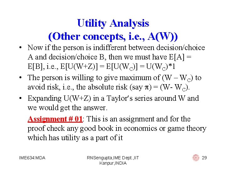
Utility Analysis (Other concepts, i. e. , A(W)) • Now if the person is indifferent between decision/choice A and decision/choice B, then we must have E[A] = E[B], i. e. , E[U(W+Z)] = E[U(WC)] = U(WC)*1 • The person is willing to give maximum of (W – WC) to avoid risk, i. e. , the absolute risk (say ) = (W- WC). • Expanding U(W+Z) in a Taylor s series around W and we would get the answer. Assignment # 01: This is an assignment and for the proof check any good book in economics or game theory which has utility as a part of it IME 634: MDA RNSengupta, IME Dept. , IIT Kanpur, INDIA 29

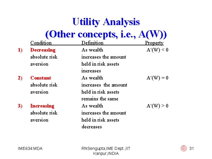
Utility Analysis (Other concepts, i. e. , A(W)) For the three different types of persons § Decreasing absolute risk aversion A (W) = d. A(W)/d(W) < 0 § Constant absolute risk aversion A (W) = d. A(W)/d(W) = 0 § Increasing absolute risk aversion A (W) = d. A(W)/d(W) > 0 IME 634: MDA RNSengupta, IME Dept. , IIT Kanpur, INDIA 30

Utility Analysis (Other concepts, i. e. , A(W)) 1) Condition Decreasing absolute risk aversion 2) Constant absolute risk aversion 3) Increasing absolute risk aversion IME 634: MDA Definition As wealth increases the amount held in risk assets increases As wealth increases the amount held in risk assets remains the same As wealth increases the amount held in risk assets decreases RNSengupta, IME Dept. , IIT Kanpur, INDIA Property A (W) < 0 A (W) = 0 A (W) > 0 31

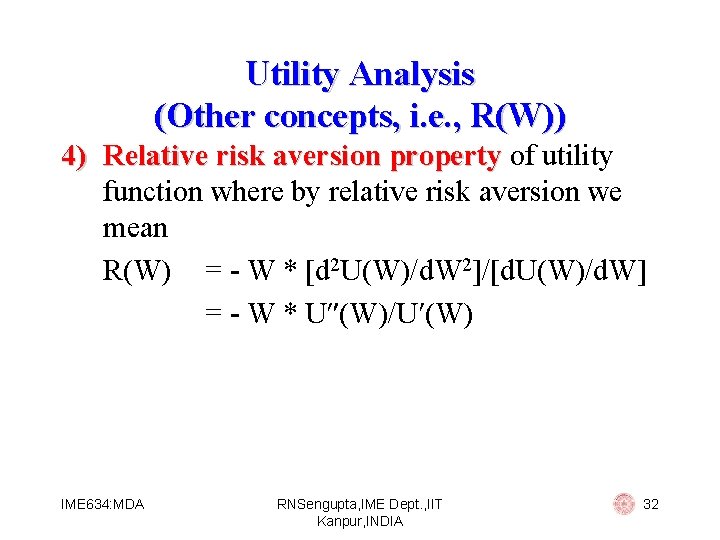
Utility Analysis (Other concepts, i. e. , R(W)) 4) Relative risk aversion property of utility function where by relative risk aversion we mean R(W) = - W * [d 2 U(W)/d. W 2]/[d. U(W)/d. W] = - W * U (W)/U (W) IME 634: MDA RNSengupta, IME Dept. , IIT Kanpur, INDIA 32

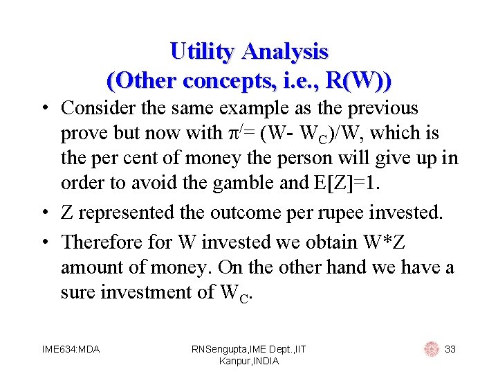
Utility Analysis (Other concepts, i. e. , R(W)) • Consider the same example as the previous prove but now with /= (W- WC)/W, which is the per cent of money the person will give up in order to avoid the gamble and E[Z]=1. • Z represented the outcome per rupee invested. • Therefore for W invested we obtain W*Z amount of money. On the other hand we have a sure investment of WC. IME 634: MDA RNSengupta, IME Dept. , IIT Kanpur, INDIA 33

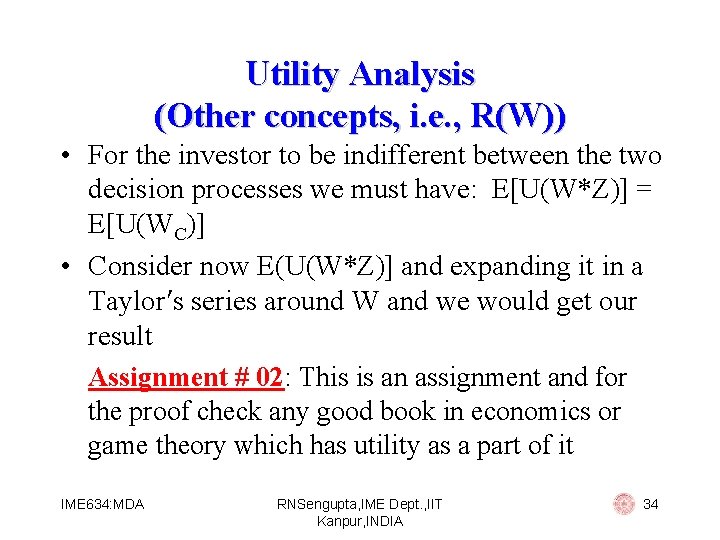
Utility Analysis (Other concepts, i. e. , R(W)) • For the investor to be indifferent between the two decision processes we must have: E[U(W*Z)] = E[U(WC)] • Consider now E(U(W*Z)] and expanding it in a Taylor s series around W and we would get our result Assignment # 02: This is an assignment and for the proof check any good book in economics or game theory which has utility as a part of it IME 634: MDA RNSengupta, IME Dept. , IIT Kanpur, INDIA 34

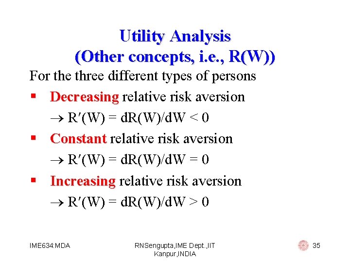
Utility Analysis (Other concepts, i. e. , R(W)) For the three different types of persons § Decreasing relative risk aversion R (W) = d. R(W)/d. W < 0 § Constant relative risk aversion R (W) = d. R(W)/d. W = 0 § Increasing relative risk aversion R (W) = d. R(W)/d. W > 0 IME 634: MDA RNSengupta, IME Dept. , IIT Kanpur, INDIA 35

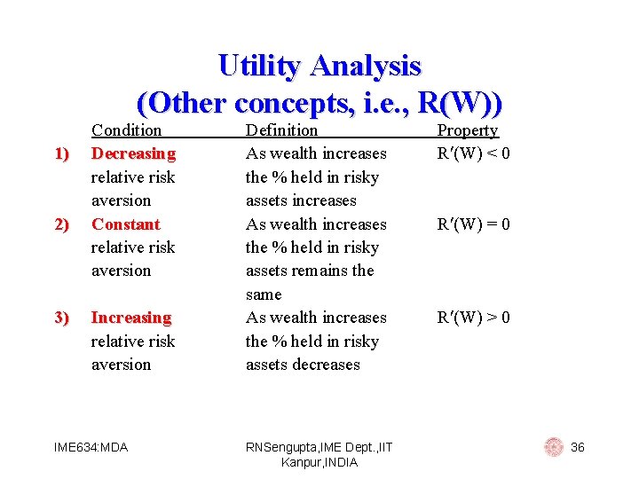
Utility Analysis (Other concepts, i. e. , R(W)) 1) 2) 3) Condition Decreasing relative risk aversion Constant relative risk aversion Increasing relative risk aversion IME 634: MDA Definition As wealth increases the % held in risky assets increases As wealth increases the % held in risky assets remains the same As wealth increases the % held in risky assets decreases RNSengupta, IME Dept. , IIT Kanpur, INDIA Property R (W) < 0 R (W) = 0 R (W) > 0 36

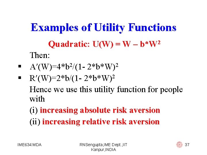
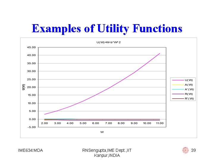
Examples of Utility Functions Quadratic: U(W) = W – b*W 2 Then: § A (W)=4*b 2/(1 - 2*b*W)2 § R (W)=2*b/(1 - 2*b*W)2 Hence we use this utility function for people with (i) increasing absolute risk aversion (ii) increasing relative risk aversion IME 634: MDA RNSengupta, IME Dept. , IIT Kanpur, INDIA 37

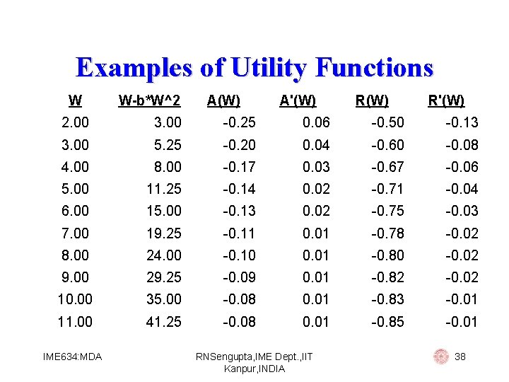
Examples of Utility Functions W W-b*W^2 A(W) A'(W) R'(W) 2. 00 3. 00 -0. 25 0. 06 -0. 50 -0. 13 3. 00 5. 25 -0. 20 0. 04 -0. 60 -0. 08 4. 00 8. 00 -0. 17 0. 03 -0. 67 -0. 06 5. 00 11. 25 -0. 14 0. 02 -0. 71 -0. 04 6. 00 15. 00 -0. 13 0. 02 -0. 75 -0. 03 7. 00 19. 25 -0. 11 0. 01 -0. 78 -0. 02 8. 00 24. 00 -0. 10 0. 01 -0. 80 -0. 02 9. 00 29. 25 -0. 09 0. 01 -0. 82 -0. 02 10. 00 35. 00 -0. 08 0. 01 -0. 83 -0. 01 11. 00 41. 25 -0. 08 0. 01 -0. 85 -0. 01 IME 634: MDA RNSengupta, IME Dept. , IIT Kanpur, INDIA 38

Examples of Utility Functions IME 634: MDA RNSengupta, IME Dept. , IIT Kanpur, INDIA 39

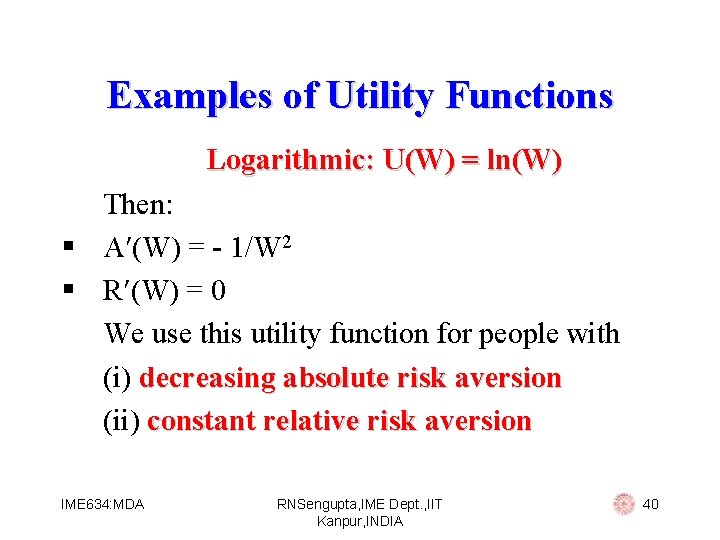
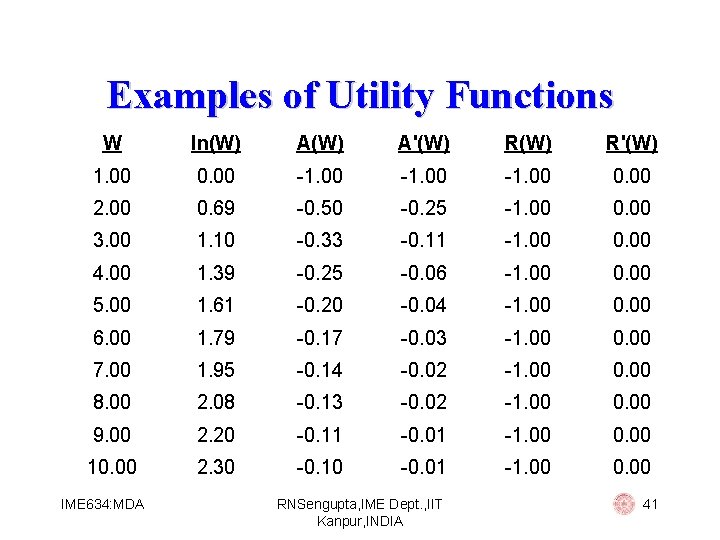
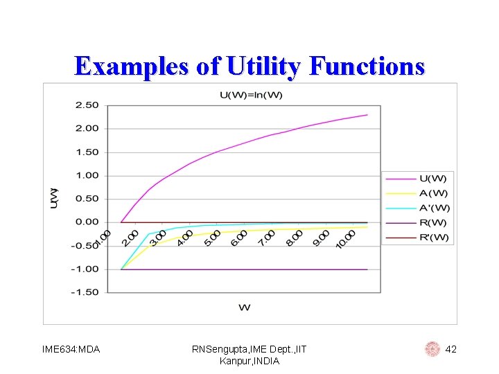
Examples of Utility Functions Logarithmic: U(W) = ln(W) Then: § A (W) = - 1/W 2 § R (W) = 0 We use this utility function for people with (i) decreasing absolute risk aversion (ii) constant relative risk aversion IME 634: MDA RNSengupta, IME Dept. , IIT Kanpur, INDIA 40

Examples of Utility Functions W ln(W) A'(W) R'(W) 1. 00 0. 00 -1. 00 0. 00 2. 00 0. 69 -0. 50 -0. 25 -1. 00 0. 00 3. 00 1. 10 -0. 33 -0. 11 -1. 00 0. 00 4. 00 1. 39 -0. 25 -0. 06 -1. 00 0. 00 5. 00 1. 61 -0. 20 -0. 04 -1. 00 0. 00 6. 00 1. 79 -0. 17 -0. 03 -1. 00 0. 00 7. 00 1. 95 -0. 14 -0. 02 -1. 00 0. 00 8. 00 2. 08 -0. 13 -0. 02 -1. 00 0. 00 9. 00 2. 20 -0. 11 -0. 01 -1. 00 0. 00 10. 00 2. 30 -0. 10 -0. 01 -1. 00 0. 00 IME 634: MDA RNSengupta, IME Dept. , IIT Kanpur, INDIA 41

Examples of Utility Functions IME 634: MDA RNSengupta, IME Dept. , IIT Kanpur, INDIA 42

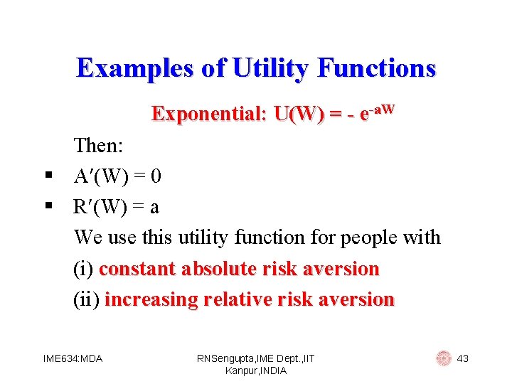
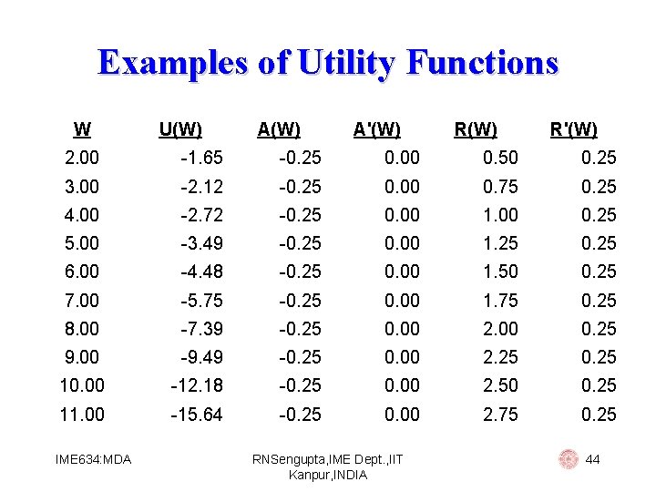
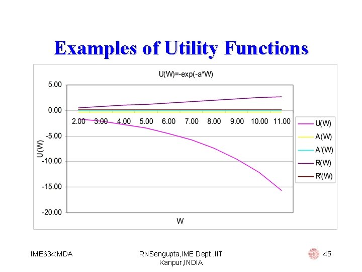
Examples of Utility Functions Exponential: U(W) = - e-a. W Then: § A (W) = 0 § R (W) = a We use this utility function for people with (i) constant absolute risk aversion (ii) increasing relative risk aversion IME 634: MDA RNSengupta, IME Dept. , IIT Kanpur, INDIA 43

Examples of Utility Functions W U(W) A'(W) R'(W) 2. 00 -1. 65 -0. 25 0. 00 0. 50 0. 25 3. 00 -2. 12 -0. 25 0. 00 0. 75 0. 25 4. 00 -2. 72 -0. 25 0. 00 1. 00 0. 25 5. 00 -3. 49 -0. 25 0. 00 1. 25 0. 25 6. 00 -4. 48 -0. 25 0. 00 1. 50 0. 25 7. 00 -5. 75 -0. 25 0. 00 1. 75 0. 25 8. 00 -7. 39 -0. 25 0. 00 2. 00 0. 25 9. 00 -9. 49 -0. 25 0. 00 2. 25 0. 25 10. 00 -12. 18 -0. 25 0. 00 2. 50 0. 25 11. 00 -15. 64 -0. 25 0. 00 2. 75 0. 25 IME 634: MDA RNSengupta, IME Dept. , IIT Kanpur, INDIA 44

Examples of Utility Functions IME 634: MDA RNSengupta, IME Dept. , IIT Kanpur, INDIA 45

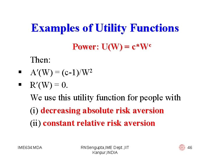
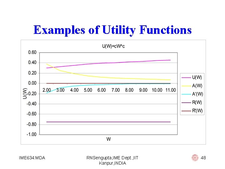
Examples of Utility Functions Power: U(W) = c*Wc Then: § A (W) = (c-1)/W 2 § R (W) = 0. We use this utility function for people with (i) decreasing absolute risk aversion (ii) constant relative risk aversion IME 634: MDA RNSengupta, IME Dept. , IIT Kanpur, INDIA 46

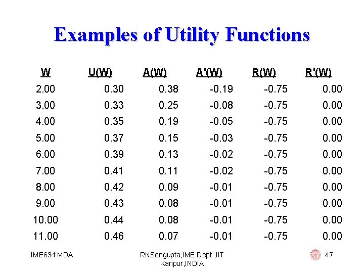
Examples of Utility Functions W U(W) A'(W) R'(W) 2. 00 0. 38 -0. 19 -0. 75 0. 00 3. 00 0. 33 0. 25 -0. 08 -0. 75 0. 00 4. 00 0. 35 0. 19 -0. 05 -0. 75 0. 00 5. 00 0. 37 0. 15 -0. 03 -0. 75 0. 00 6. 00 0. 39 0. 13 -0. 02 -0. 75 0. 00 7. 00 0. 41 0. 11 -0. 02 -0. 75 0. 00 8. 00 0. 42 0. 09 -0. 01 -0. 75 0. 00 9. 00 0. 43 0. 08 -0. 01 -0. 75 0. 00 10. 00 0. 44 0. 08 -0. 01 -0. 75 0. 00 11. 00 0. 46 0. 07 -0. 01 -0. 75 0. 00 IME 634: MDA RNSengupta, IME Dept. , IIT Kanpur, INDIA 47

Examples of Utility Functions IME 634: MDA RNSengupta, IME Dept. , IIT Kanpur, INDIA 48

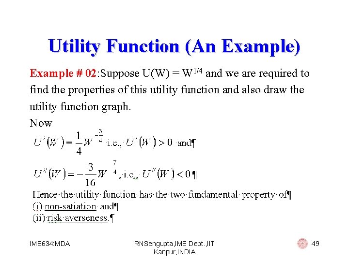
Utility Function (An Example) Example # 02: Suppose U(W) = W 1/4 and we are required to find the properties of this utility function and also draw the utility function graph. Now IME 634: MDA RNSengupta, IME Dept. , IIT Kanpur, INDIA 49

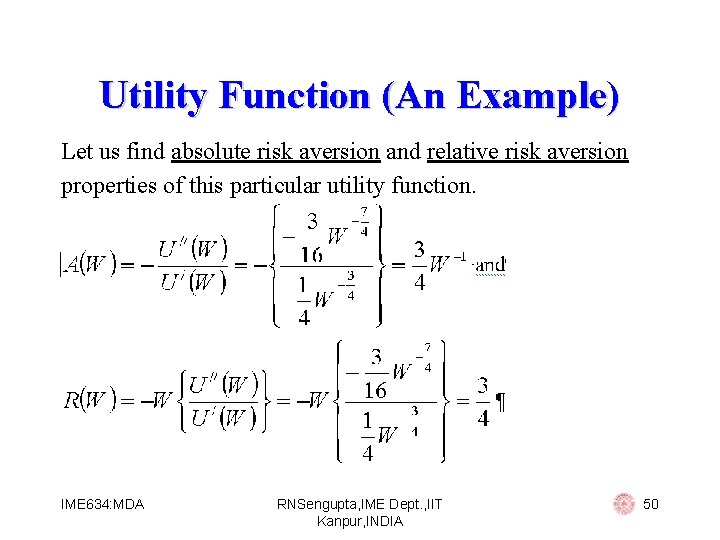
Utility Function (An Example) Let us find absolute risk aversion and relative risk aversion properties of this particular utility function. IME 634: MDA RNSengupta, IME Dept. , IIT Kanpur, INDIA 50

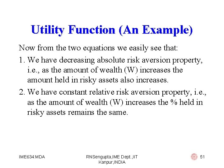
Utility Function (An Example) Now from the two equations we easily see that: 1. We have decreasing absolute risk aversion property, i. e. , as the amount of wealth (W) increases the amount held in risky assets also increases. 2. We have constant relative risk aversion property, i. e. , as the amount of wealth (W) increases the % held in risky assets remains the same. IME 634: MDA RNSengupta, IME Dept. , IIT Kanpur, INDIA 51

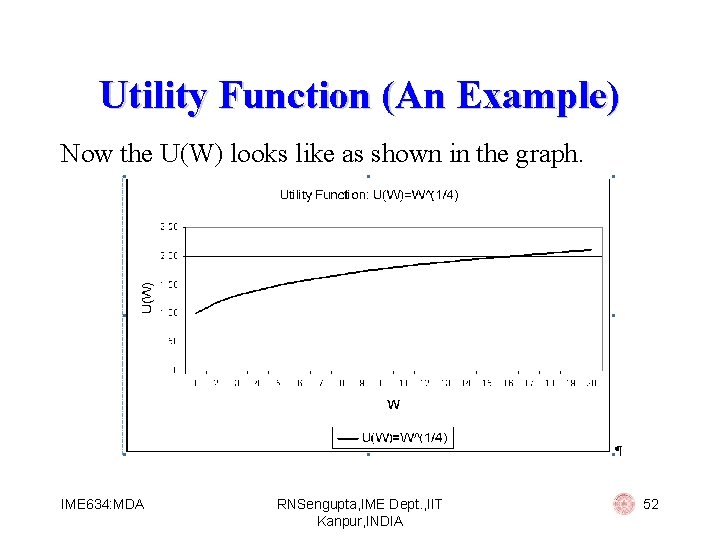
Utility Function (An Example) Now the U(W) looks like as shown in the graph. IME 634: MDA RNSengupta, IME Dept. , IIT Kanpur, INDIA 52

Utility Analysis The actual value of expected utility is of no use, except when comparing with other alternatives. Hence we use an important concept of certainty equivalent, equivalent which is the amount of certain wealth (risk free) that has the utility level exactly equal to this expected utility value. We define U(C) = E[U(W)], where C is the certainty value IME 634: MDA RNSengupta, IME Dept. , IIT Kanpur, INDIA 53

Utility Analysis § § How is this value of certainty equivalent (C) useful Suppose that we have a decision process with a set of outcomes, their probabilities and the corresponding utility values. In case we want to compare this decision process we can find the certainty equivalent so that comparison is easier. To find the exact form of the utility function for a person who is not clear about the form of utility function he/she uses. IME 634: MDA RNSengupta, IME Dept. , IIT Kanpur, INDIA 54

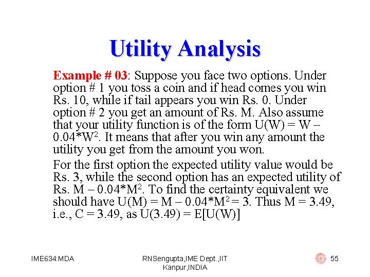
Utility Analysis Example # 03: Suppose you face two options. Under option # 1 you toss a coin and if head comes you win Rs. 10, while if tail appears you win Rs. 0. Under option # 2 you get an amount of Rs. M. Also assume that your utility function is of the form U(W) = W – 0. 04*W 2. It means that after you win any amount the utility you get from the amount you won. For the first option the expected utility value would be Rs. 3, while the second option has an expected utility of Rs. M – 0. 04*M 2. To find the certainty equivalent we should have U(M) = M – 0. 04*M 2 = 3. Thus M = 3. 49, i. e. , C = 3. 49, as U(3. 49) = E[U(W)] IME 634: MDA RNSengupta, IME Dept. , IIT Kanpur, INDIA 55

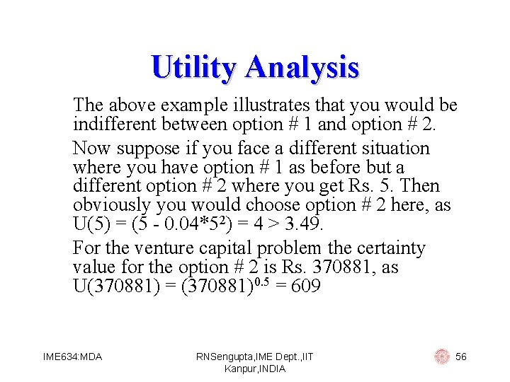
Utility Analysis The above example illustrates that you would be indifferent between option # 1 and option # 2. Now suppose if you face a different situation where you have option # 1 as before but a different option # 2 where you get Rs. 5. Then obviously you would choose option # 2 here, as U(5) = (5 - 0. 04*52) = 4 > 3. 49. For the venture capital problem the certainty value for the option # 2 is Rs. 370881, as U(370881) = (370881)0. 5 = 609 IME 634: MDA RNSengupta, IME Dept. , IIT Kanpur, INDIA 56

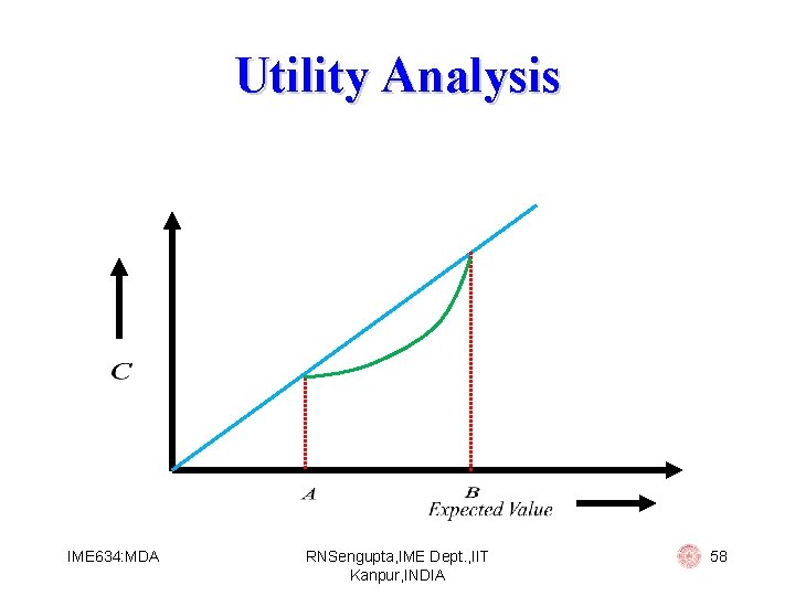
Utility Analysis § A risk averse person will select a equivalent certain event rather than the gamble § A risk neutral person will be indifferent between the equivalent certain event and the gamble § A risk seeking person will select the gamble rather than the equivalent certain event IME 634: MDA RNSengupta, IME Dept. , IIT Kanpur, INDIA 57

Utility Analysis IME 634: MDA RNSengupta, IME Dept. , IIT Kanpur, INDIA 58

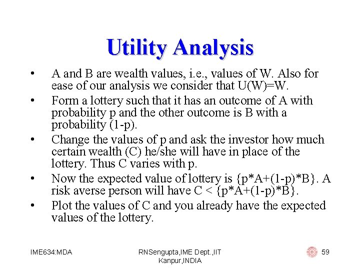
Utility Analysis • • • A and B are wealth values, i. e. , values of W. Also for ease of our analysis we consider that U(W)=W. Form a lottery such that it has an outcome of A with probability p and the other outcome is B with a probability (1 -p). Change the values of p and ask the investor how much certain wealth (C) he/she will have in place of the lottery. Thus C varies with p. Now the expected value of lottery is {p*A+(1 -p)*B}. A risk averse person will have C < {p*A+(1 -p)*B}. Plot the values of C and you already have the expected values of the lottery. IME 634: MDA RNSengupta, IME Dept. , IIT Kanpur, INDIA 59

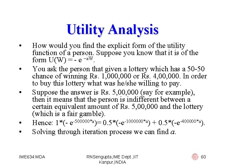
Utility Analysis • • • How would you find the explicit form of the utility function of a person. Suppose you know that it is of the form U(W) = - e –a. W. You ask the person that given a lottery which has a 50 -50 chance of winning Rs. 1, 000 or Rs. 4, 000. In order to buy this lottery what was he/she willing to pay. Suppose the answer is Rs. 5, 000 (say for example), then it means that the person is indifferent between a certain equivalent amount of Rs. 5, 000 and the lottery (which is a fair gamble). Hence: 1*(- e-500000*a)= 0. 5*(-e-1000000*a) + 0. 5*(-e-400000*a). Solving through iteration process we can find a. IME 634: MDA RNSengupta, IME Dept. , IIT Kanpur, INDIA 60

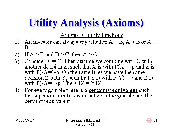
Utility Analysis (Axioms) 1) 2) 3) 4) Axioms of utility functions An investor can always say whether A = B, A > B or A < B If A > B and B > C, then A > C Consider X = Y. Then assume we combine with X with another decision Z, such that X is with P(X) = p and Z is with P(Z) =1 -p. On the same lines we have the same decision Z with Y, such that Y is with P(Y) = p and Z is with P(Z) = 1 -p. The X+Z = Y+Z For every gamble there is a certainty equivalent such that a person is indifferent between the gamble and the certainty equivalent IME 634: MDA RNSengupta, IME Dept. , IIT Kanpur, INDIA 61

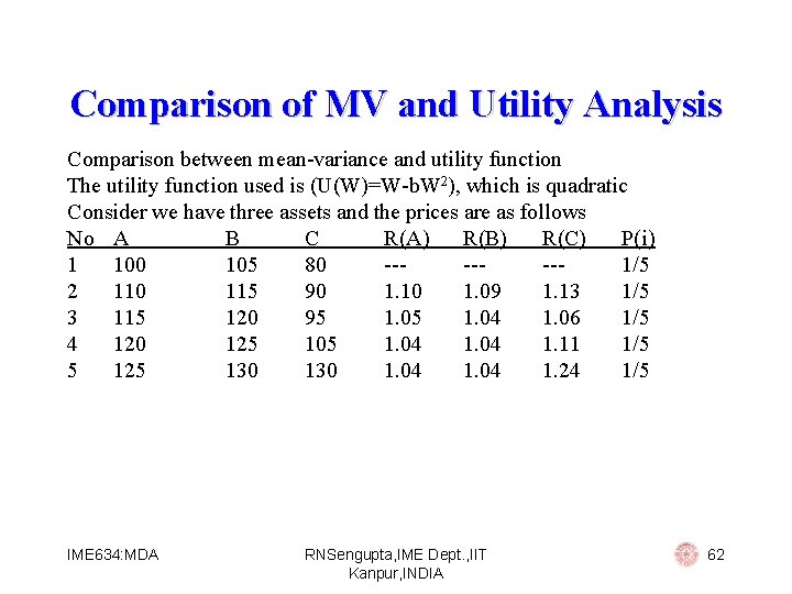
Comparison of MV and Utility Analysis Comparison between mean-variance and utility function The utility function used is (U(W)=W-b. W 2), which is quadratic Consider we have three assets and the prices are as follows No A B C R(A) R(B) R(C) P(i) 1 100 105 80 ------1/5 2 110 115 90 1. 10 1. 09 1. 13 1/5 3 115 120 95 1. 04 1. 06 1/5 4 120 125 105 1. 04 1. 11 1/5 5 125 130 1. 04 1. 24 1/5 IME 634: MDA RNSengupta, IME Dept. , IIT Kanpur, INDIA 62

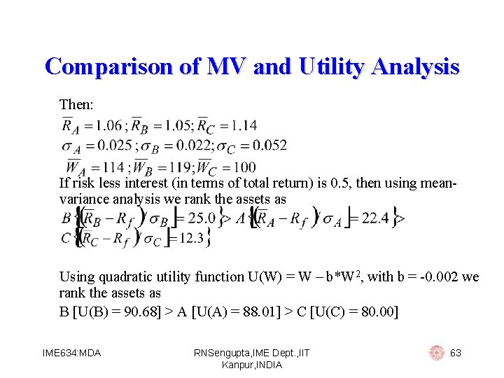
Comparison of MV and Utility Analysis Then: If risk less interest (in terms of total return) is 0. 5, then using meanvariance analysis we rank the assets as Using quadratic utility function U(W) = W – b*W 2, with b = -0. 002 we rank the assets as B [U(B) = 90. 68] > A [U(A) = 88. 01] > C [U(C) = 80. 00] IME 634: MDA RNSengupta, IME Dept. , IIT Kanpur, INDIA 63

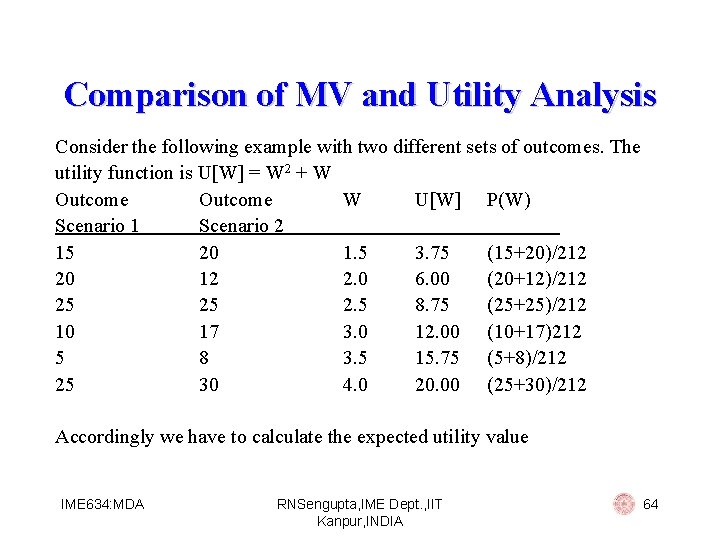
Comparison of MV and Utility Analysis Consider the following example with two different sets of outcomes. The utility function is U[W] = W 2 + W Outcome W U[W] P(W) Scenario 1 Scenario 2 15 20 1. 5 3. 75 (15+20)/212 20 12 2. 0 6. 00 (20+12)/212 25 25 2. 5 8. 75 (25+25)/212 10 17 3. 0 12. 00 (10+17)212 5 8 3. 5 15. 75 (5+8)/212 25 30 4. 0 20. 00 (25+30)/212 Accordingly we have to calculate the expected utility value IME 634: MDA RNSengupta, IME Dept. , IIT Kanpur, INDIA 64

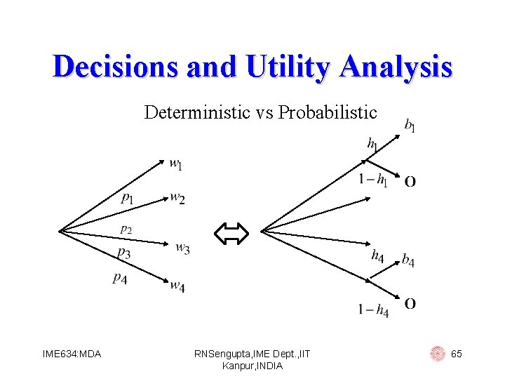
Decisions and Utility Analysis Deterministic vs Probabilistic IME 634: MDA RNSengupta, IME Dept. , IIT Kanpur, INDIA 65

Decisions and Utility Analysis § § People have other criteria for investment/project/portfolio solutions and they are Geometric mean return Safety first criteria Stochastic dominance Analysis in terms of characteristics of the return distribution IME 634: MDA RNSengupta, IME Dept. , IIT Kanpur, INDIA 66

Decisions and Utility Analysis Geometric mean return For the selection process we consider the maximum GM has: § The highest probability of reaching or exceeding any given wealth level in the shortest possible time. § The highest probability of exceeding any given wealth level over any given period of time IME 634: MDA RNSengupta, IME Dept. , IIT Kanpur, INDIA 67

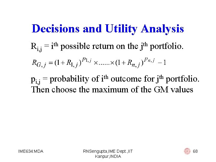
Decisions and Utility Analysis Ri, j = ith possible return on the jth portfolio. pi, j = probability of ith outcome for jth portfolio. Then choose the maximum of the GM values IME 634: MDA RNSengupta, IME Dept. , IIT Kanpur, INDIA 68

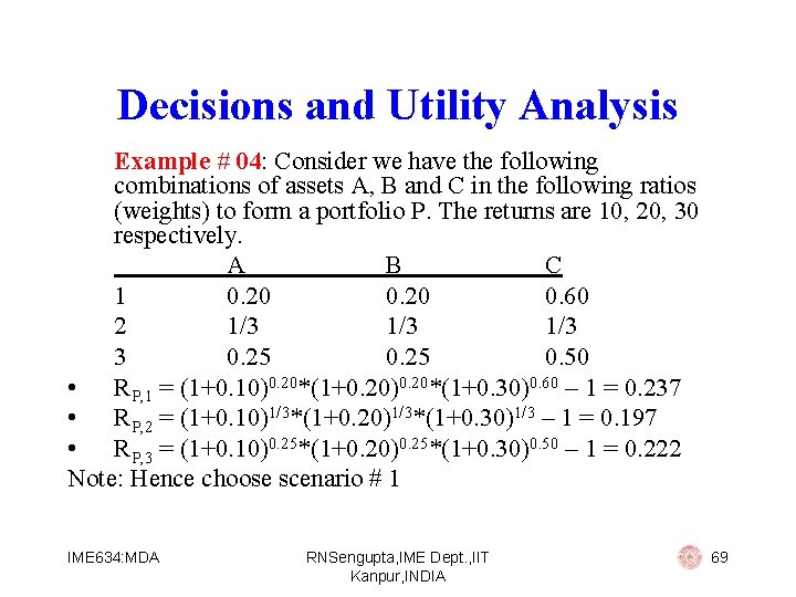
Decisions and Utility Analysis Example # 04: Consider we have the following combinations of assets A, B and C in the following ratios (weights) to form a portfolio P. The returns are 10, 20, 30 respectively. A B C 1 0. 20 0. 60 2 1/3 1/3 3 0. 25 0. 50 • RP, 1 = (1+0. 10)0. 20*(1+0. 20)0. 20*(1+0. 30)0. 60 – 1 = 0. 237 • RP, 2 = (1+0. 10)1/3*(1+0. 20)1/3*(1+0. 30)1/3 – 1 = 0. 197 • RP, 3 = (1+0. 10)0. 25*(1+0. 20)0. 25*(1+0. 30)0. 50 – 1 = 0. 222 Note: Hence choose scenario # 1 IME 634: MDA RNSengupta, IME Dept. , IIT Kanpur, INDIA 69

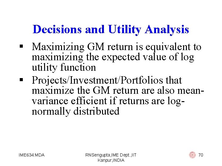
Decisions and Utility Analysis § Maximizing GM return is equivalent to maximizing the expected value of log utility function § Projects/Investment/Portfolios that maximize the GM return are also meanvariance efficient if returns are lognormally distributed IME 634: MDA RNSengupta, IME Dept. , IIT Kanpur, INDIA 70

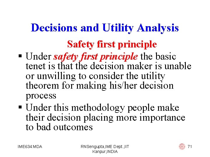
Decisions and Utility Analysis Safety first principle § Under safety first principle the basic tenet is that the decision maker is unable or unwilling to consider the utility theorem for making his/her decision process § Under this methodology people make their decision placing more importance to bad outcomes IME 634: MDA RNSengupta, IME Dept. , IIT Kanpur, INDIA 71

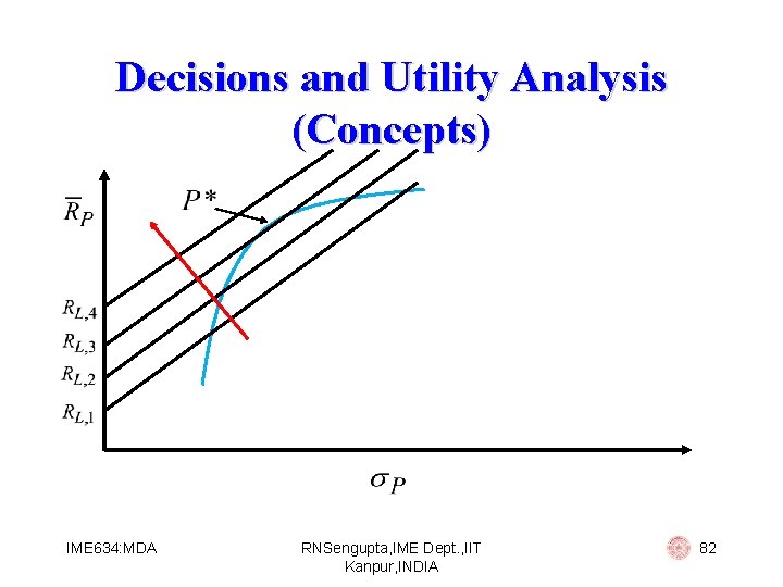
Decisions and Utility Analysis (Concepts) Safety first principles (rules) § Min Pr[RP<RL] § Max RL § IME 634: MDA RNSengupta, IME Dept. , IIT Kanpur, INDIA 72

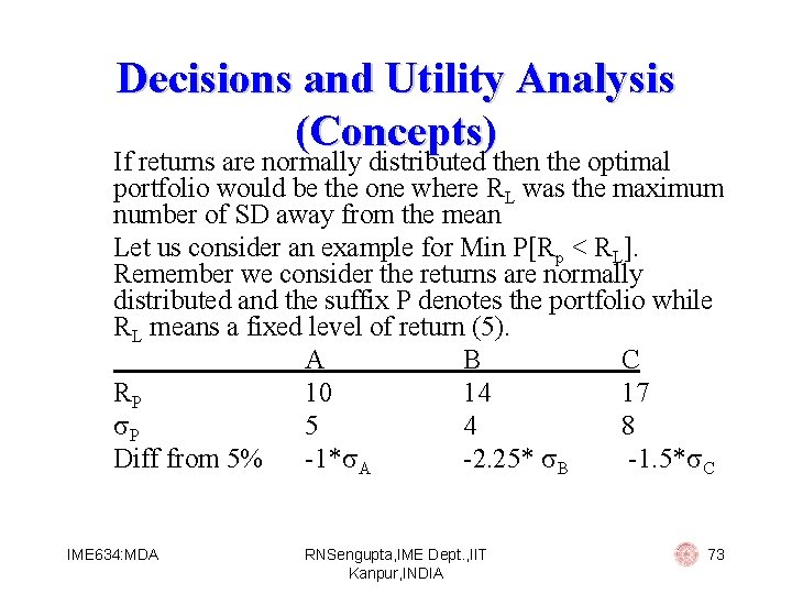
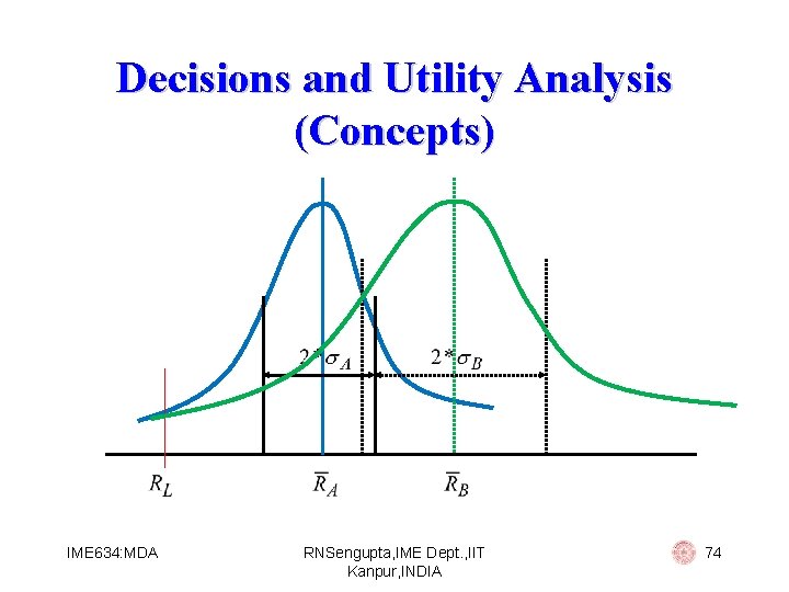
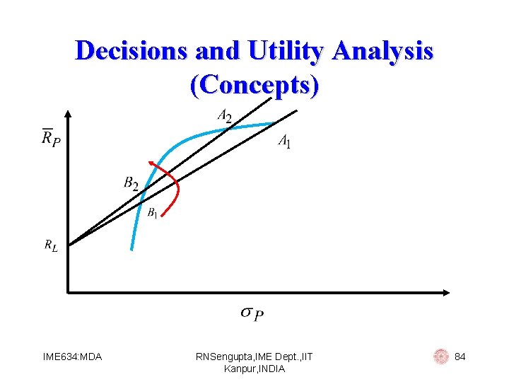
Decisions and Utility Analysis (Concepts) If returns are normally distributed then the optimal portfolio would be the one where RL was the maximum number of SD away from the mean Let us consider an example for Min P[Rp < RL]. Remember we consider the returns are normally distributed and the suffix P denotes the portfolio while RL means a fixed level of return (5). A B C RP 10 14 17 P 5 4 8 Diff from 5% -1* A -2. 25* B -1. 5* C IME 634: MDA RNSengupta, IME Dept. , IIT Kanpur, INDIA 73

Decisions and Utility Analysis (Concepts) IME 634: MDA RNSengupta, IME Dept. , IIT Kanpur, INDIA 74

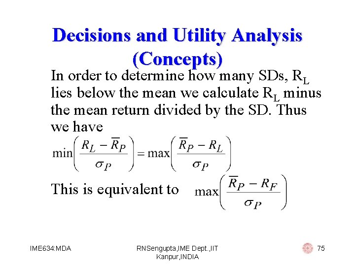
Decisions and Utility Analysis (Concepts) In order to determine how many SDs, RL lies below the mean we calculate RL minus the mean return divided by the SD. Thus we have This is equivalent to IME 634: MDA RNSengupta, IME Dept. , IIT Kanpur, INDIA 75

Decisions and Utility Analysis (Concepts) Even though for our example we have simplified our assumption by considering only normal distribution, but this would hold for any distributions having first and second moments. IME 634: MDA RNSengupta, IME Dept. , IIT Kanpur, INDIA 76

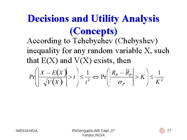
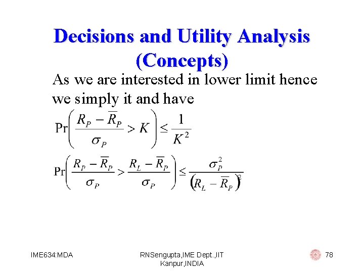
Decisions and Utility Analysis (Concepts) According to Tchebychev (Chebyshev) inequality for any random variable X, such that E(X) and V(X) exists, then IME 634: MDA RNSengupta, IME Dept. , IIT Kanpur, INDIA 77

Decisions and Utility Analysis (Concepts) As we are interested in lower limit hence we simply it and have IME 634: MDA RNSengupta, IME Dept. , IIT Kanpur, INDIA 78

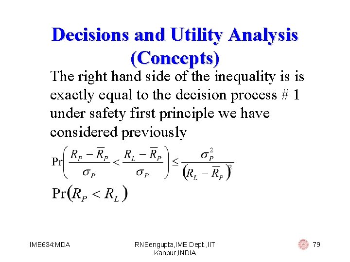
Decisions and Utility Analysis (Concepts) The right hand side of the inequality is is exactly equal to the decision process # 1 under safety first principle we have considered previously IME 634: MDA RNSengupta, IME Dept. , IIT Kanpur, INDIA 79

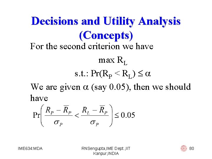
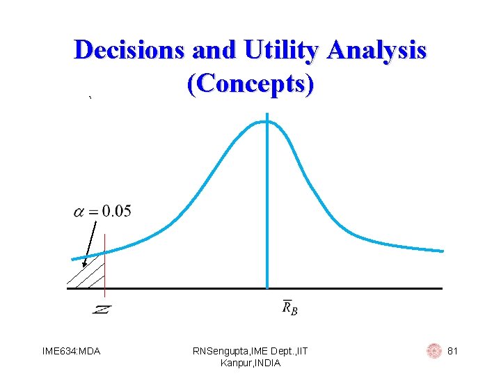
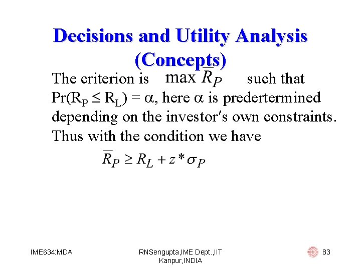
Decisions and Utility Analysis (Concepts) For the second criterion we have max RL s. t. : Pr(RP < RL) We are given (say 0. 05), then we should have IME 634: MDA RNSengupta, IME Dept. , IIT Kanpur, INDIA 80

Decisions and Utility Analysis (Concepts) ` IME 634: MDA RNSengupta, IME Dept. , IIT Kanpur, INDIA 81

Decisions and Utility Analysis (Concepts) IME 634: MDA RNSengupta, IME Dept. , IIT Kanpur, INDIA 82

Decisions and Utility Analysis (Concepts) The criterion is such that Pr(RP RL) = , here is predertermined depending on the investor s own constraints. Thus with the condition we have IME 634: MDA RNSengupta, IME Dept. , IIT Kanpur, INDIA 83

Decisions and Utility Analysis (Concepts) IME 634: MDA RNSengupta, IME Dept. , IIT Kanpur, INDIA 84

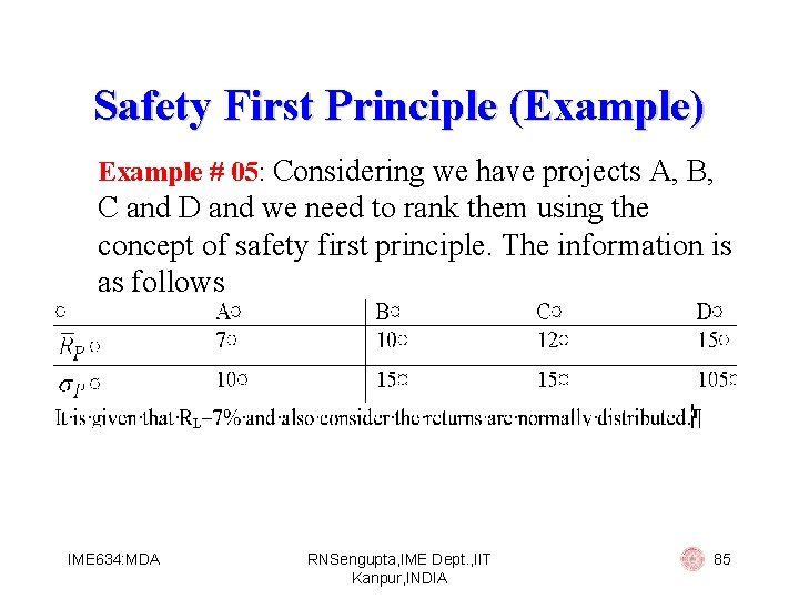
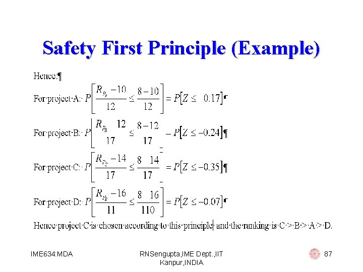
Safety First Principle (Example) Example # 05: Considering we have projects A, B, C and D and we need to rank them using the concept of safety first principle. The information is as follows IME 634: MDA RNSengupta, IME Dept. , IIT Kanpur, INDIA 85

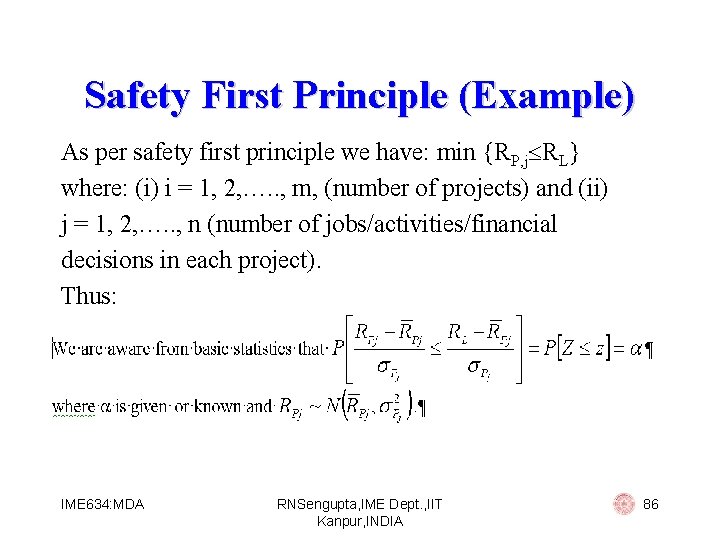
Safety First Principle (Example) As per safety first principle we have: min {RP, j RL} where: (i) i = 1, 2, …. . , m, (number of projects) and (ii) j = 1, 2, …. . , n (number of jobs/activities/financial decisions in each project). Thus: IME 634: MDA RNSengupta, IME Dept. , IIT Kanpur, INDIA 86

Safety First Principle (Example) IME 634: MDA RNSengupta, IME Dept. , IIT Kanpur, INDIA 87

Stochastic Dominance • First-order stochastic dominance • Second-order stochastic dominance • Third-order stochastic dominance IME 634: MDA RNSengupta, IME Dept. , IIT Kanpur, INDIA 88

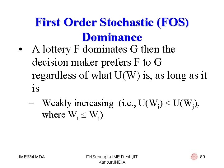
First Order Stochastic (FOS) Dominance • A lottery F dominates G then the decision maker prefers F to G regardless of what U(W) is, as long as it is – Weakly increasing (i. e. , U(Wi) U(Wj), where Wi Wj) IME 634: MDA RNSengupta, IME Dept. , IIT Kanpur, INDIA 89

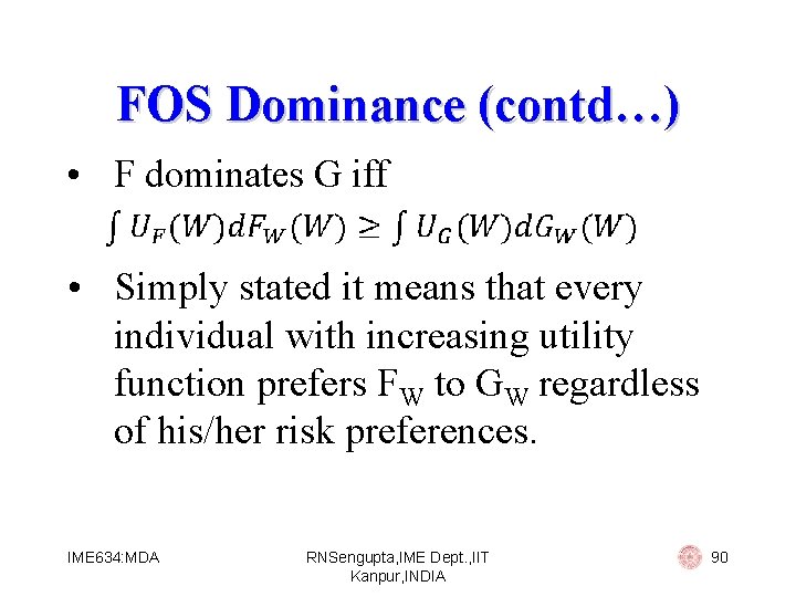
FOS Dominance (contd…) • F dominates G iff • Simply stated it means that every individual with increasing utility function prefers FW to GW regardless of his/her risk preferences. IME 634: MDA RNSengupta, IME Dept. , IIT Kanpur, INDIA 90

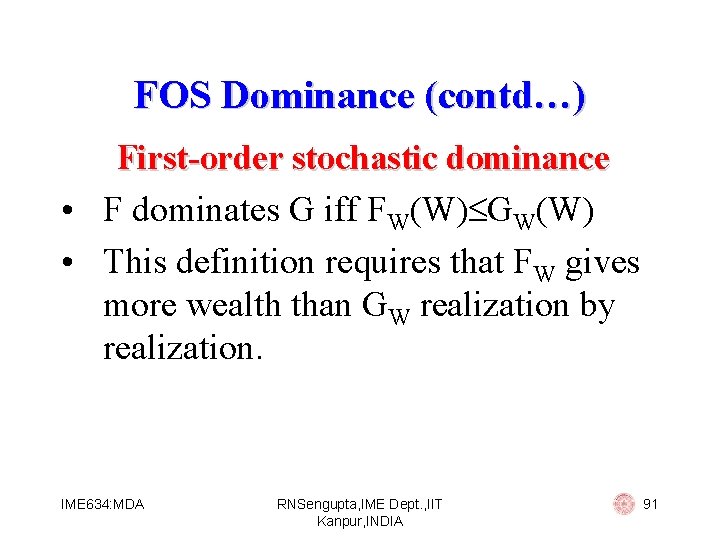
FOS Dominance (contd…) First-order stochastic dominance • F dominates G iff FW(W) GW(W) • This definition requires that FW gives more wealth than GW realization by realization. IME 634: MDA RNSengupta, IME Dept. , IIT Kanpur, INDIA 91

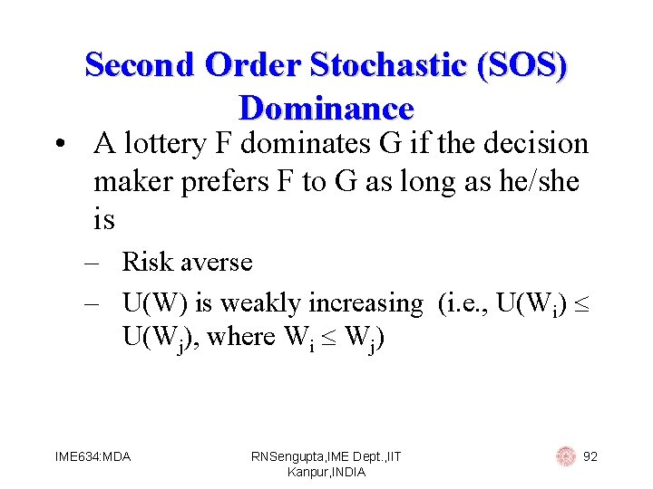
Second Order Stochastic (SOS) Dominance • A lottery F dominates G if the decision maker prefers F to G as long as he/she is – Risk averse – U(W) is weakly increasing (i. e. , U(Wi) U(Wj), where Wi Wj) IME 634: MDA RNSengupta, IME Dept. , IIT Kanpur, INDIA 92

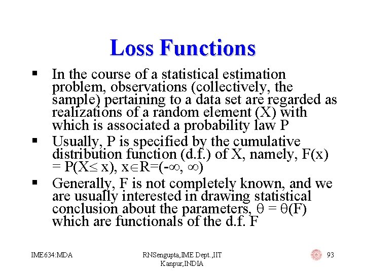
Loss Functions § In the course of a statistical estimation problem, observations (collectively, the sample) pertaining to a data set are regarded as realizations of a random element (X) with which is associated a probability law P § Usually, P is specified by the cumulative distribution function (d. f. ) of X, namely, F(x) = P(X x), x R=(- , ) § Generally, F is not completely known, and we are usually interested in drawing statistical conclusion about the parameters, = (F) which are functionals of the d. f. F IME 634: MDA RNSengupta, IME Dept. , IIT Kanpur, INDIA 93

Loss Functions (contd…) § In a parametric model, the assumed functional form of F may involve some unknown algebraic constant(s), which are interpreted as the parameters, e. g. , in the normal d. f. , the algebraic constants are themselves the mean ( ) and the variance ( 2) § The objective in point estimation is to utilize the information in the given set (X 1, …. . , Xn) of sample observations (random variables) to choose a suitable statistic Tn = T(X 1, X 2, . . …, Xn) such that Tn estimates (parameter) in a meaningful way IME 634: MDA RNSengupta, IME Dept. , IIT Kanpur, INDIA 94

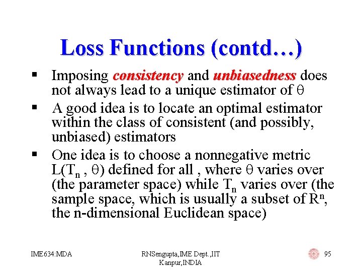
Loss Functions (contd…) § Imposing consistency and unbiasedness does not always lead to a unique estimator of § A good idea is to locate an optimal estimator within the class of consistent (and possibly, unbiased) estimators § One idea is to choose a nonnegative metric L(Tn , ) defined for all , where varies over (the parameter space) while Tn varies over (the sample space, which is usually a subset of Rn, the n-dimensional Euclidean space) IME 634: MDA RNSengupta, IME Dept. , IIT Kanpur, INDIA 95

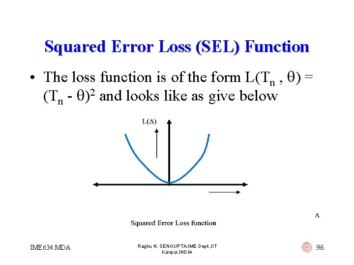
Squared Error Loss (SEL) Function • The loss function is of the form L(Tn , ) = (Tn - )2 and looks like as give below IME 634: MDA Raghu N. SENGUPTA, IME Dept. , IIT Kanpur, INDIA 96

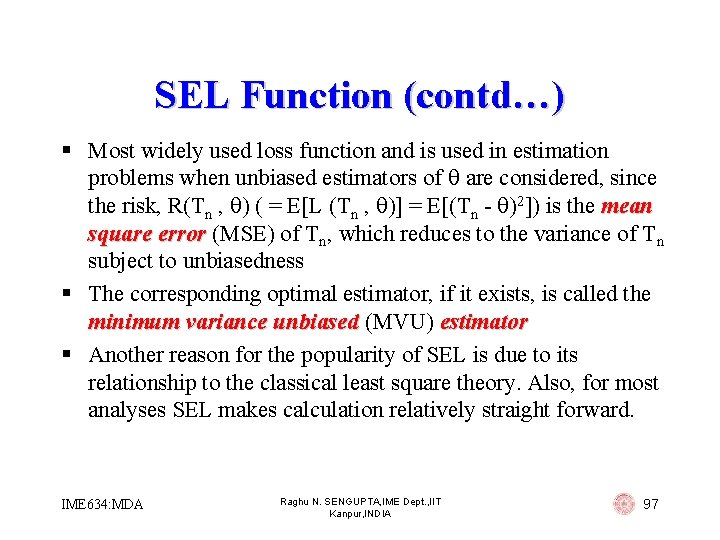
SEL Function (contd…) § Most widely used loss function and is used in estimation problems when unbiased estimators of are considered, since the risk, R(Tn , ) ( = E[L (Tn , )] = E[(Tn - )2]) is the mean square error (MSE) of Tn, which reduces to the variance of Tn subject to unbiasedness § The corresponding optimal estimator, if it exists, is called the minimum variance unbiased (MVU) estimator § Another reason for the popularity of SEL is due to its relationship to the classical least square theory. Also, for most analyses SEL makes calculation relatively straight forward. IME 634: MDA Raghu N. SENGUPTA, IME Dept. , IIT Kanpur, INDIA 97

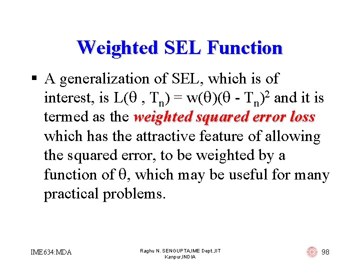
Weighted SEL Function § A generalization of SEL, which is of interest, is L( , Tn) = w( )( - Tn)2 and it is termed as the weighted squared error loss which has the attractive feature of allowing the squared error, to be weighted by a function of , which may be useful for many practical problems. IME 634: MDA Raghu N. SENGUPTA, IME Dept. , IIT Kanpur, INDIA 98

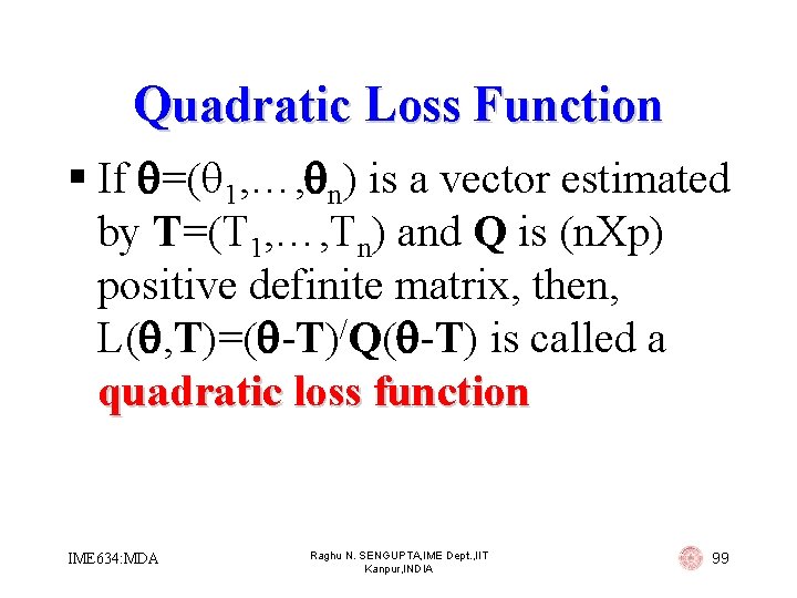
Quadratic Loss Function § If =( 1, …, n) is a vector estimated by T=(T 1, …, Tn) and Q is (n. Xp) positive definite matrix, then, L( , T)=( -T)/Q( -T) is called a quadratic loss function IME 634: MDA Raghu N. SENGUPTA, IME Dept. , IIT Kanpur, INDIA 99

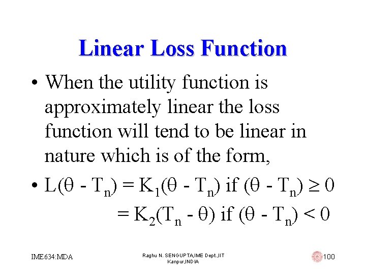
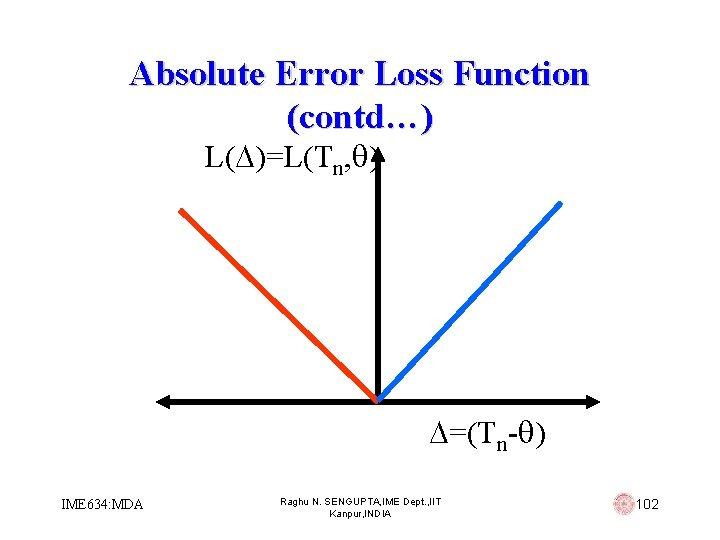
Linear Loss Function • When the utility function is approximately linear the loss function will tend to be linear in nature which is of the form, • L( - Tn) = K 1( - Tn) if ( - Tn) 0 = K 2(Tn - ) if ( - Tn) < 0 IME 634: MDA Raghu N. SENGUPTA, IME Dept. , IIT Kanpur, INDIA 100

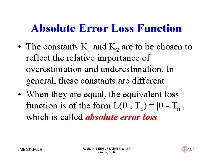
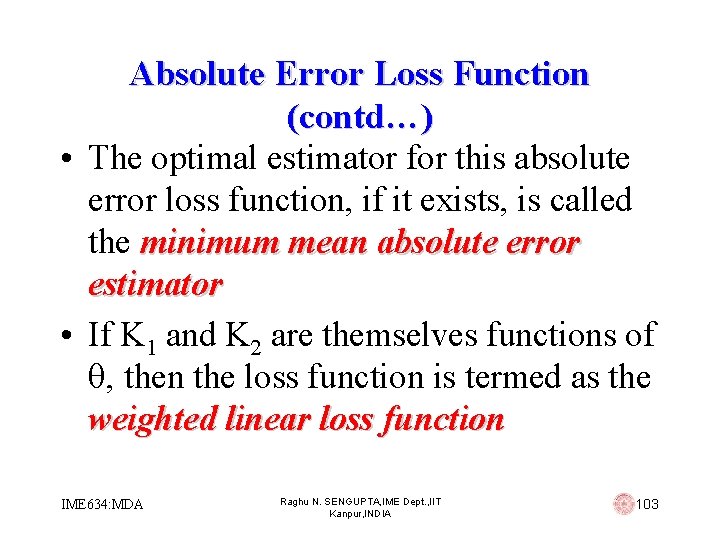
Absolute Error Loss Function • The constants K 1 and K 2 are to be chosen to reflect the relative importance of overestimation and underestimation. In general, these constants are different • When they are equal, the equivalent loss function is of the form L( , Tn) = | - Tn|, which is called absolute error loss IME 634: MDA Raghu N. SENGUPTA, IME Dept. , IIT Kanpur, INDIA 101

Absolute Error Loss Function (contd…) L( )=L(Tn, ) =(Tn- ) IME 634: MDA Raghu N. SENGUPTA, IME Dept. , IIT Kanpur, INDIA 102

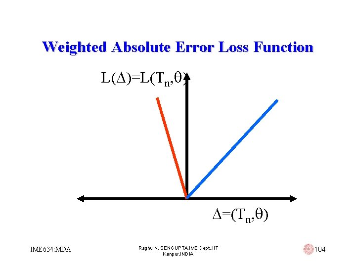
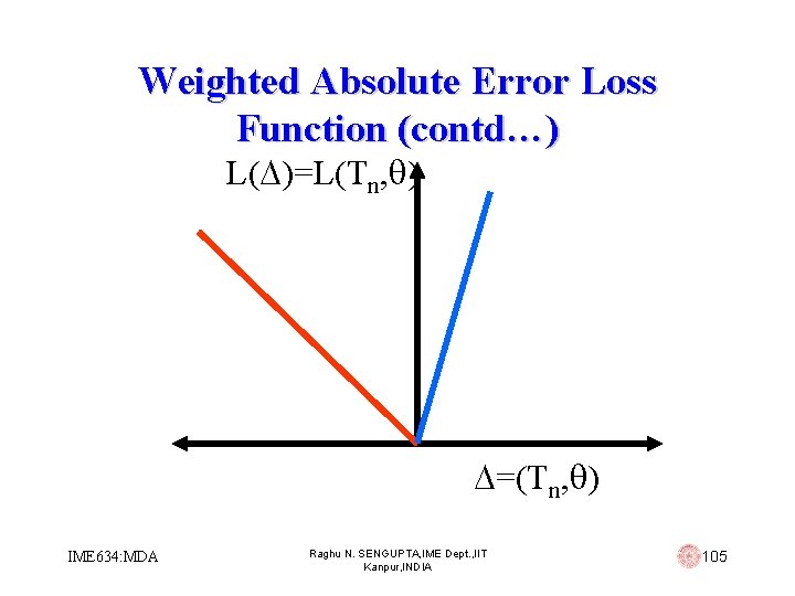
Absolute Error Loss Function (contd…) • The optimal estimator for this absolute error loss function, if it exists, is called the minimum mean absolute error estimator • If K 1 and K 2 are themselves functions of , then the loss function is termed as the weighted linear loss function IME 634: MDA Raghu N. SENGUPTA, IME Dept. , IIT Kanpur, INDIA 103

Weighted Absolute Error Loss Function L( )=L(Tn, ) =(Tn, ) IME 634: MDA Raghu N. SENGUPTA, IME Dept. , IIT Kanpur, INDIA 104

Weighted Absolute Error Loss Function (contd…) L( )=L(Tn, ) =(Tn, ) IME 634: MDA Raghu N. SENGUPTA, IME Dept. , IIT Kanpur, INDIA 105

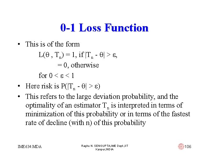
0 -1 Loss Function • This is of the form L( , Tn) = 1, if |Tn - | > , = 0, otherwise for 0 < < 1 • Here risk is P(|Tn - | > ) • This refers to the large deviation probability, and the optimality of an estimator Tn is interpreted in terms of minimization of this probability or in terms of the fastest rate of decline (with n) of this probability IME 634: MDA Raghu N. SENGUPTA, IME Dept. , IIT Kanpur, INDIA 106

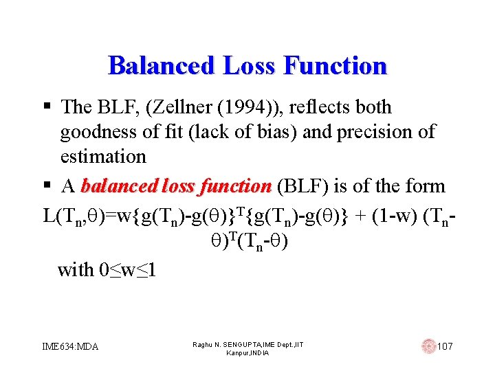
Balanced Loss Function § The BLF, (Zellner (1994)), reflects both goodness of fit (lack of bias) and precision of estimation § A balanced loss function (BLF) is of the form L(Tn, )=w{g(Tn)-g( )}T{g(Tn)-g( )} + (1 -w) (Tn )T(Tn- ) with 0≤w≤ 1 IME 634: MDA Raghu N. SENGUPTA, IME Dept. , IIT Kanpur, INDIA 107

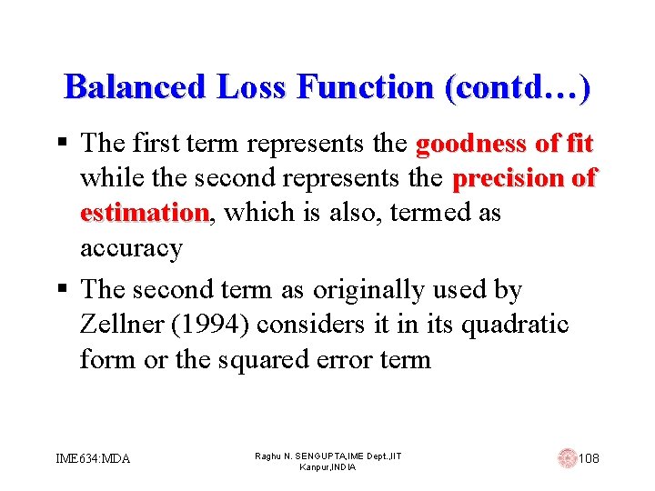
Balanced Loss Function (contd…) § The first term represents the goodness of fit while the second represents the precision of estimation, estimation which is also, termed as accuracy § The second term as originally used by Zellner (1994) considers it in its quadratic form or the squared error term IME 634: MDA Raghu N. SENGUPTA, IME Dept. , IIT Kanpur, INDIA 108

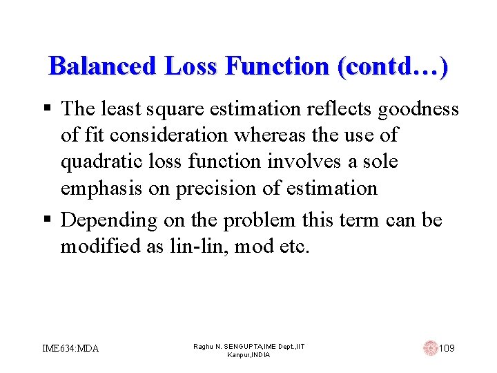
Balanced Loss Function (contd…) § The least square estimation reflects goodness of fit consideration whereas the use of quadratic loss function involves a sole emphasis on precision of estimation § Depending on the problem this term can be modified as lin-lin, mod etc. IME 634: MDA Raghu N. SENGUPTA, IME Dept. , IIT Kanpur, INDIA 109

Linear Exponential (LINEX) Loss Function § The fact the overestimation and underestimation of may be of unequal consequence has not been properly or adequately emphasized in any of the above loss functions § Varian (1975) first employs such a loss function in real-estate assessment IME 634: MDA Raghu N. SENGUPTA, IME Dept. , IIT Kanpur, INDIA 110

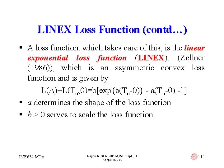
LINEX Loss Function (contd…) § A loss function, which takes care of this, is the linear exponential loss function (LINEX), (Zellner LINEX (1986)), which is an asymmetric convex loss function and is given by L( )=L(Tn, )=b[exp{a(Tn- )} - a(Tn- ) -1] § a determines the shape of the loss function § b > 0 serves to scale the loss function IME 634: MDA Raghu N. SENGUPTA, IME Dept. , IIT Kanpur, INDIA 111

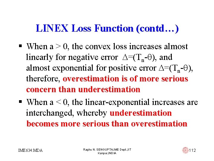
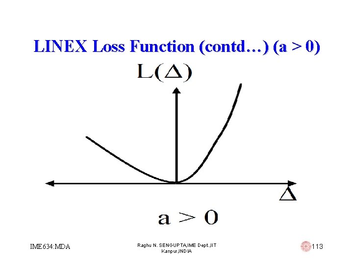
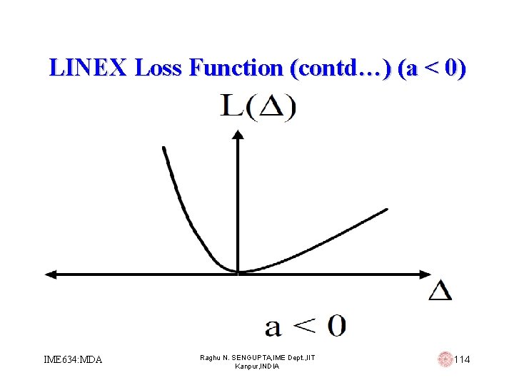
LINEX Loss Function (contd…) § When a > 0, the convex loss increases almost linearly for negative error =(Tn- ), and almost exponential for positive error =(Tn- ), therefore, overestimation is of more serious concern than underestimation § When a < 0, the linear-exponential increases are interchanged, whereby underestimation becomes more serious than overestimation IME 634: MDA Raghu N. SENGUPTA, IME Dept. , IIT Kanpur, INDIA 112

LINEX Loss Function (contd…) (a > 0) IME 634: MDA Raghu N. SENGUPTA, IME Dept. , IIT Kanpur, INDIA 113

LINEX Loss Function (contd…) (a < 0) IME 634: MDA Raghu N. SENGUPTA, IME Dept. , IIT Kanpur, INDIA 114

LINEX Loss Function: Example # 01 § Consider a company plans to launch a new product, say a refrigerator in the consumer market § Also suppose that similar products from different manufacturers already exist in the market IME 634: MDA Raghu N. SENGUPTA, IME Dept. , IIT Kanpur, INDIA 115

LINEX Loss Function: Example # 01 (contd…) § Then the company is expected to give some warranty for the particular product, i. e. , the refrigerator, to its customers in order to sell the product § Now if the value of this warranty is more than the average time of failure for the product, then the aforesaid mentioned company needs to replace the damaged products it sells, or face litigation charges IME 634: MDA Raghu N. SENGUPTA, IME Dept. , IIT Kanpur, INDIA 116

LINEX Loss Function: Example # 01 (contd…) § On the other if the warranty period is less than the average failure time of similar products available in the market, then the company losses the market share to its rivals, as naturally, customers are willing to buy the refrigerator from the competitors who assure a higher warranty period IME 634: MDA Raghu N. SENGUPTA, IME Dept. , IIT Kanpur, INDIA 117

LINEX Loss Function: Example # 01 (contd…) § Under such a situation it is definitely advisable to estimate the warranty life time using an asymmetric loss § What values of a one should use would then depend on the level of importance our company places on overestimation versus underestimation, i. e. , the cost of litigation versus the cost of a loss in the market share of the company IME 634: MDA Raghu N. SENGUPTA, IME Dept. , IIT Kanpur, INDIA 118

LINEX Loss Function: Example # 02 § As a second example, assume a civil engineer is building a dam and he/she is interested in finding the height of the dam which is being built § If due to some error the height is estimated to be greater than the actual value then the cost the engineer incurs are mainly due to material and labour IME 634: MDA Raghu N. SENGUPTA, IME Dept. , IIT Kanpur, INDIA 119

LINEX Loss Function: Example # 02 (contd…) § On the other hand, if the estimated height is less than what it should be, then the consequences can be disastrous in terms of an environmental impact, which in monetary terms can be very high § So it is logical to use a value of a < 0 in such situations such that underestimation is penalized more than over estimation IME 634: MDA Raghu N. SENGUPTA, IME Dept. , IIT Kanpur, INDIA 120

LINEX Loss Function: Example # 03 § Finally to illustrate the significance of over estimation when compared with underestimation let us consider a different real life example § Consider an electrical company manufactures vacuum circuit breakers/interrupters, which are used as a fuse in high voltage system IME 634: MDA Raghu N. SENGUPTA, IME Dept. , IIT Kanpur, INDIA 121

LINEX Loss Function: Example # 03 (contd…) § As for any product these circuit breakers have a working life and it is of utmost importance that this value is estimated as accurately as possible IME 634: MDA Raghu N. SENGUPTA, IME Dept. , IIT Kanpur, INDIA 122

LINEX Loss Function: Example # 03 (contd…) § In case they are underestimated than what its value is in reality, then the consequences is just labour and man hour loss in terms of production stoppage time IME 634: MDA Raghu N. SENGUPTA, IME Dept. , IIT Kanpur, INDIA 123

LINEX Loss Function: Example # 03 (contd…) § On the other hand if the working life of the circuit breaker is over estimated than the actual figure, then it would definitely signify an exponential form of loss in monetary terms due to an accident or major break down of machineries § So, for these categories of practical estimation problems we always consider a > 0 IME 634: MDA Raghu N. SENGUPTA, IME Dept. , IIT Kanpur, INDIA 124