IME 634 Management Decision Analysis Raghu Nandan Sengupta

IME 634: Management Decision Analysis Raghu Nandan Sengupta Industrial & Management Department Indian Institute of Technology Kanpur IME 634: MDA R. N. Sengupta, IME Dept. , IIT Kanpur 1

Data Analysis Regression and Forecasting IME 634: MDA R. N. Sengupta, IME Dept. , IIT Kanpur 2

Regression and Forecasting Topics to be covered Linear regression, Multiple linear regression, Curve fitting, Variability in data due to time dependence/independence, etc. , Concept of forecasting, etc. IME 634: MDA R. N. Sengupta, IME Dept. , IIT Kanpur 3

Regression and Forecasting 1) Forecasting 2) Prediction 3) Different types of Regression 4) Curve Fitting IME 634: MDA R. N. Sengupta, IME Dept. , IIT Kanpur 4

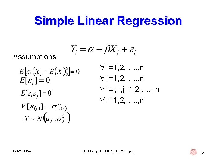
Simple Linear Regression Under this method the most important assumption is that the dependent variable, which we denote by Y is due to effect of only one independent variable, which we denote by X IME 634: MDA R. N. Sengupta, IME Dept. , IIT Kanpur 5

Simple Linear Regression Assumptions i=1, 2, …. . , n i j, i, j=1, 2, …. . , n i=1, 2, …. . , n IME 634: MDA R. N. Sengupta, IME Dept. , IIT Kanpur 6

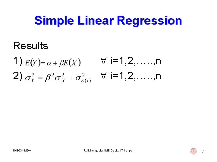
Simple Linear Regression Results 1) 2) IME 634: MDA i=1, 2, …. . , n R. N. Sengupta, IME Dept. , IIT Kanpur 7

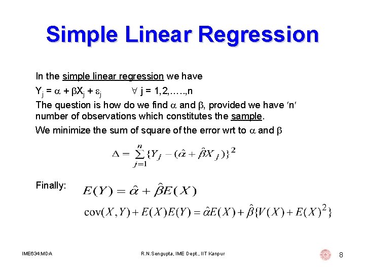
Simple Linear Regression In the simple linear regression we have Yj = + Xj + j j = 1, 2, …. . , n The question is how do we find and , provided we have n number of observations which constitutes the sample. We minimize the sum of square of the error wrt to and Finally: IME 634: MDA R. N. Sengupta, IME Dept. , IIT Kanpur 8

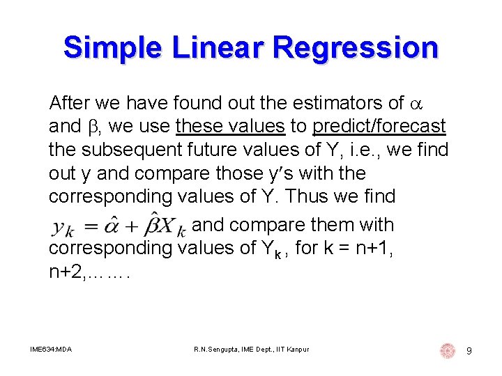
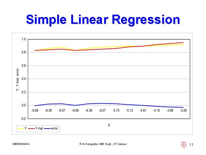
Simple Linear Regression After we have found out the estimators of and , we use these values to predict/forecast the subsequent future values of Y, i. e. , we find out y and compare those y s with the corresponding values of Y. Thus we find and compare them with corresponding values of Yk , for k = n+1, n+2, ……. IME 634: MDA R. N. Sengupta, IME Dept. , IIT Kanpur 9

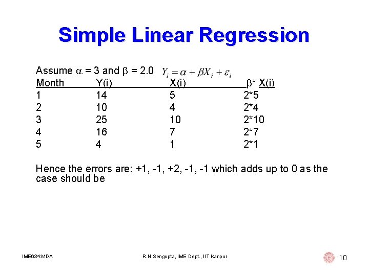
Simple Linear Regression Assume = 3 and = 2. 0 Month Y(i) 1 14 2 10 3 25 4 16 5 4 X(i) 5 4 10 7 1 * X(i) 2*5 2*4 2*10 2*7 2*1 Hence the errors are: +1, -1, +2, -1 which adds up to 0 as the case should be IME 634: MDA R. N. Sengupta, IME Dept. , IIT Kanpur 10

Simple Linear Regression IME 634: MDA R. N. Sengupta, IME Dept. , IIT Kanpur 11

Multi Linear Regression Using this methodology we try to capture the effect of other important independent variables, X 1, X 2, …. . , XK that cause movement of the dependent variable Y. It is very important to remember that all these independent variables should give maximum information about the dependent variable Y. IME 634: MDA R. N. Sengupta, IME Dept. , IIT Kanpur 12

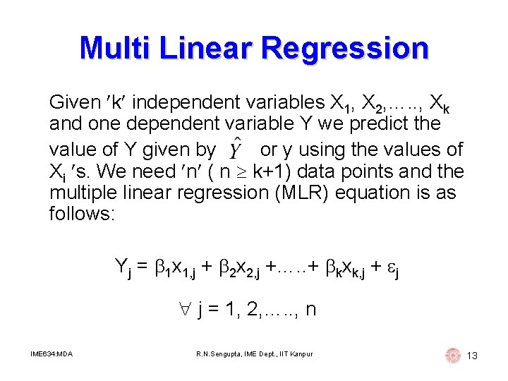
Multi Linear Regression Given k independent variables X 1, X 2, …. . , Xk and one dependent variable Y we predict the value of Y given by or y using the values of Xi s. We need n ( n k+1) data points and the multiple linear regression (MLR) equation is as follows: Yj = 1 x 1, j + 2 x 2, j +…. . + kxk, j + j j = 1, 2, …. . , n IME 634: MDA R. N. Sengupta, IME Dept. , IIT Kanpur 13

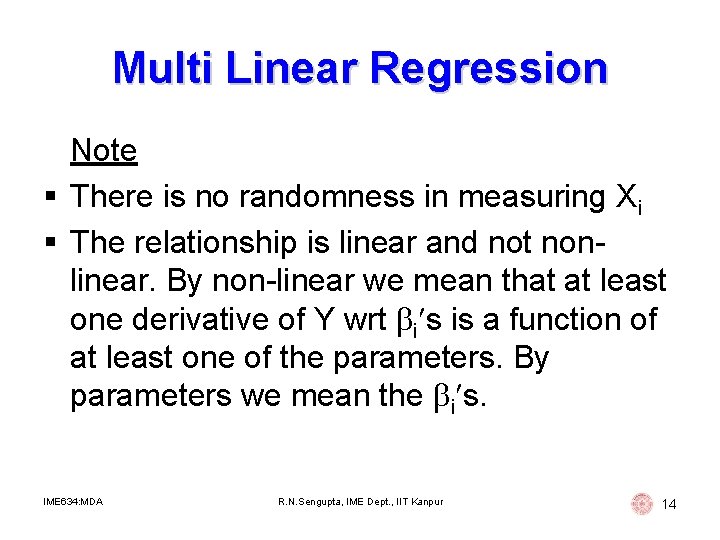
Multi Linear Regression Note § There is no randomness in measuring Xi § The relationship is linear and not nonlinear. By non-linear we mean that at least one derivative of Y wrt i s is a function of at least one of the parameters. By parameters we mean the i s. IME 634: MDA R. N. Sengupta, IME Dept. , IIT Kanpur 14

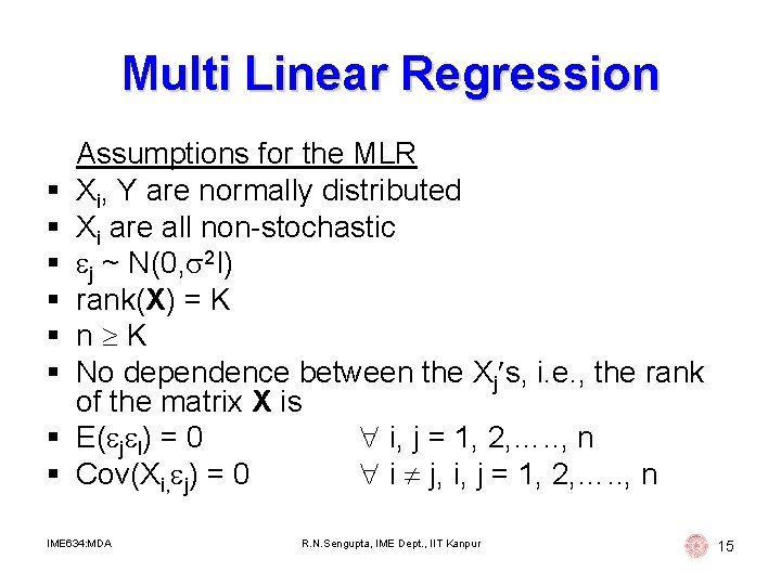
Multi Linear Regression § § § § Assumptions for the MLR Xi, Y are normally distributed Xi are all non-stochastic j ~ N(0, 2 I) rank(X) = K n K No dependence between the Xj s, i. e. , the rank of the matrix X is E( j l) = 0 i, j = 1, 2, …. . , n Cov(Xi, j) = 0 i j, i, j = 1, 2, …. . , n IME 634: MDA R. N. Sengupta, IME Dept. , IIT Kanpur 15

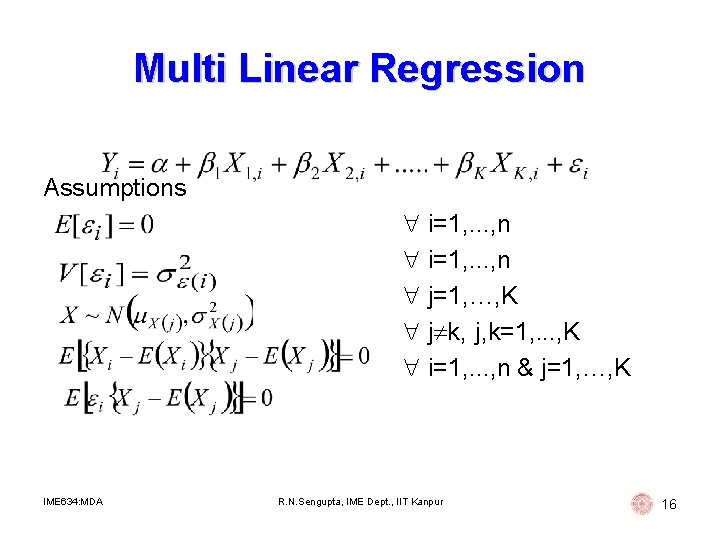
Multi Linear Regression Assumptions i=1, . . . , n j=1, …, K j k, j, k=1, . . . , K i=1, . . . , n & j=1, …, K IME 634: MDA R. N. Sengupta, IME Dept. , IIT Kanpur 16

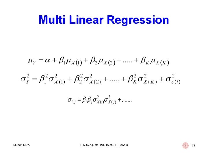
Multi Linear Regression IME 634: MDA R. N. Sengupta, IME Dept. , IIT Kanpur 17

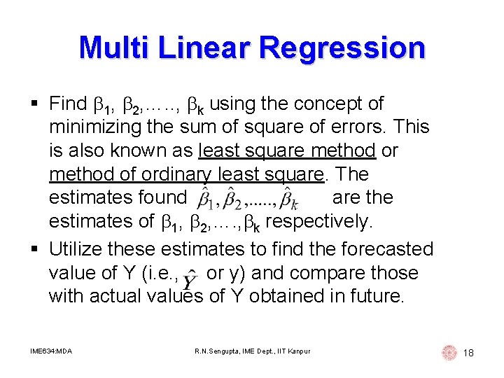
Multi Linear Regression § Find 1, 2, …. . , k using the concept of minimizing the sum of square of errors. This is also known as least square method or method of ordinary least square. The estimates found are the estimates of 1, 2, …. , k respectively. § Utilize these estimates to find the forecasted value of Y (i. e. , or y) and compare those with actual values of Y obtained in future. IME 634: MDA R. N. Sengupta, IME Dept. , IIT Kanpur 18

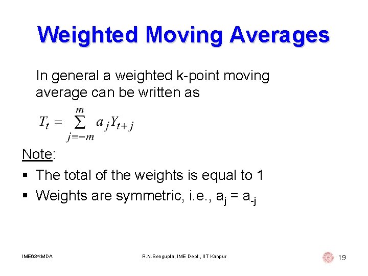
Weighted Moving Averages In general a weighted k-point moving average can be written as Note: § The total of the weights is equal to 1 § Weights are symmetric, i. e. , aj = a-j IME 634: MDA R. N. Sengupta, IME Dept. , IIT Kanpur 19

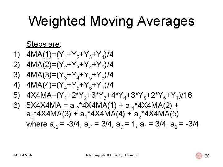
Weighted Moving Averages 1) 2) 3) 4) 5) 6) Steps are: 4 MA(1)=(Y 1+Y 2+Y 3+Y 4)/4 4 MA(2)=(Y 2+Y 3+Y 4+Y 5)/4 4 MA(3)=(Y 3+Y 4+Y 5+Y 6)/4 4 MA(4)=(Y 4+Y 5+Y 6+Y 7)/4 4 X 4 MA=(Y 1+2*Y 2+3*Y 3+4*Y 4+3*Y 5+2*Y 6+Y 7)/16 5 X 4 X 4 MA = a-2*4 X 4 MA(1) + a-1*4 X 4 MA(2) + a 0*4 X 4 MA(3) + a 1*4 X 4 MA(4) + a 2*4 X 4 MA(5) where a-2 = -3/4, a-1 = 3/4, a 0 = 1, a 1 = 3/4, a 2 = -3/4 IME 634: MDA R. N. Sengupta, IME Dept. , IIT Kanpur 20

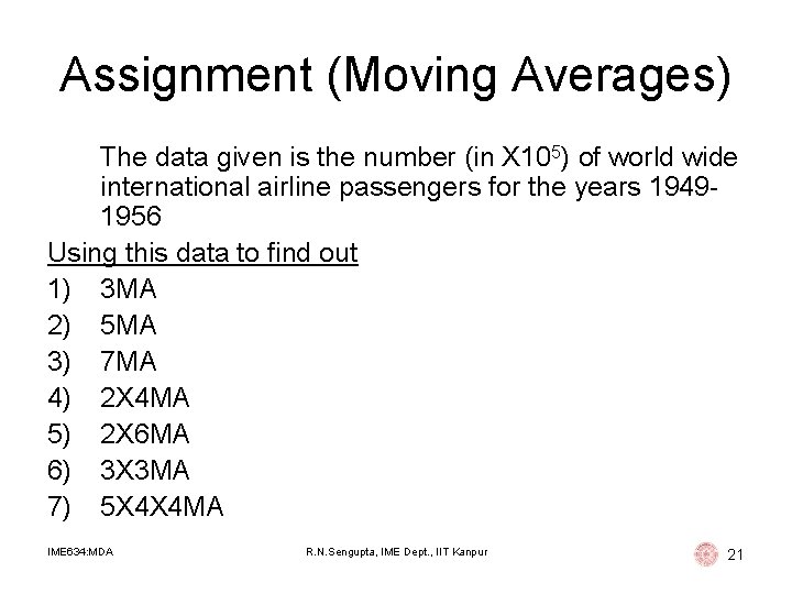
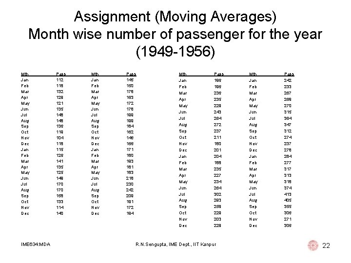
Assignment (Moving Averages) The data given is the number (in X 105) of world wide international airline passengers for the years 19491956 Using this data to find out 1) 3 MA 2) 5 MA 3) 7 MA 4) 2 X 4 MA 5) 2 X 6 MA 6) 3 X 3 MA 7) 5 X 4 X 4 MA IME 634: MDA R. N. Sengupta, IME Dept. , IIT Kanpur 21

Assignment (Moving Averages) Month wise number of passenger for the year (1949 -1956) Mth Jan Feb Mar Apr May Jun Jul Aug Sep Oct Nov Dec IME 634: MDA Pass 112 118 132 129 121 135 148 136 119 104 118 115 126 141 135 125 149 170 158 133 114 140 Mth Jan Feb Mar Apr May Jun Jul Aug Sep Oct Nov Dec Pass 145 150 178 163 172 178 199 184 162 146 166 171 180 193 181 183 218 230 242 209 191 172 194 Mth Jan Feb Mar Apr May Jun Jul Aug Sep Oct Nov Dec Pass 196 236 235 229 243 264 272 237 211 180 201 204 188 235 227 234 264 302 293 259 229 203 229 R. N. Sengupta, IME Dept. , IIT Kanpur Mth Jan Feb Mar Apr May Jun Jul Aug Sep Oct Nov Dec Pass 242 233 267 269 270 315 364 347 312 274 237 278 284 277 313 318 374 413 405 355 306 271 306 22

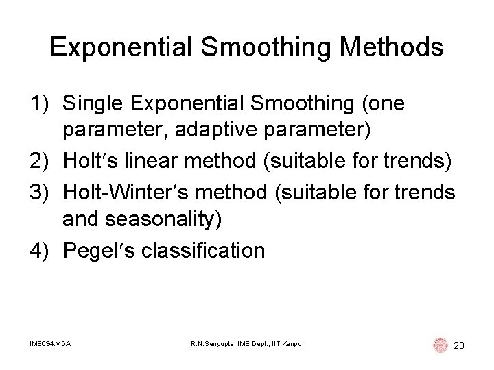
Exponential Smoothing Methods 1) Single Exponential Smoothing (one parameter, adaptive parameter) 2) Holt s linear method (suitable for trends) 3) Holt-Winter s method (suitable for trends and seasonality) 4) Pegel s classification IME 634: MDA R. N. Sengupta, IME Dept. , IIT Kanpur 23

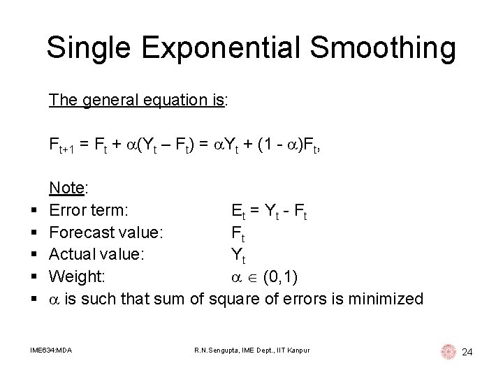
Single Exponential Smoothing The general equation is: Ft+1 = Ft + (Yt – Ft) = Yt + (1 - )Ft, § § § Note: Error term: Et = Y t - F t Forecast value: Ft Actual value: Yt Weight: (0, 1) is such that sum of square of errors is minimized IME 634: MDA R. N. Sengupta, IME Dept. , IIT Kanpur 24

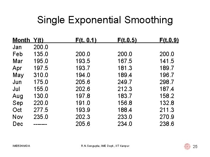
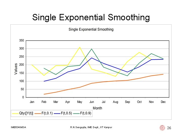
Single Exponential Smoothing Month Jan Feb Mar Apr May Jun Jul Aug Sep Oct Nov Dec IME 634: MDA Y(t) 200. 0 135. 0 197. 5 310. 0 175. 0 155. 0 130. 0 220. 0 277. 5 235. 0 ------- F(t, 0. 1) F(t. 0. 5) F(t, 0. 9) 200. 0 193. 5 193. 7 194. 0 205. 6 202. 6 197. 8 191. 0 193. 9 202. 3 205. 6 200. 0 167. 5 181. 3 189. 4 249. 7 212. 3 183. 7 156. 8 188. 4 233. 0 234. 0 200. 0 141. 5 189. 7 196. 7 298. 7 187. 4 158. 2 132. 8 211. 3 270. 9 238. 6 R. N. Sengupta, IME Dept. , IIT Kanpur 25

Single Exponential Smoothing IME 634: MDA R. N. Sengupta, IME Dept. , IIT Kanpur 26

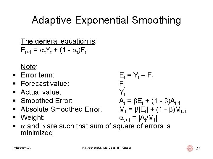
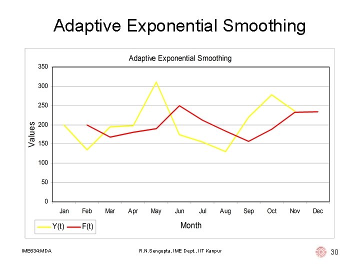
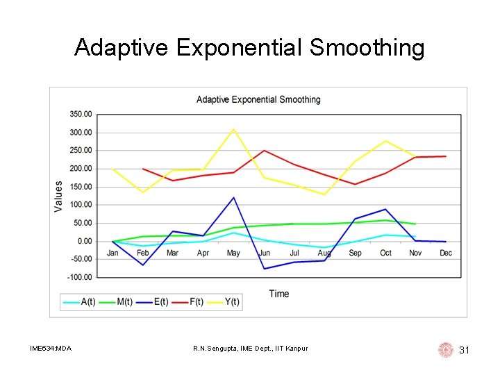
Adaptive Exponential Smoothing The general equation is: Ft+1 = t. Yt + (1 - t)Ft § § § § Note: Error term: Et = Y t – F t Forecast value: Ft Actual value: Yt Smoothed Error: At = Et + (1 - )At-1 Absolute Smoothed Error: Mt = |Et| + (1 - )Mt-1 Weight: t+1 = |At/Mt| and are such that sum of square of errors is minimized IME 634: MDA R. N. Sengupta, IME Dept. , IIT Kanpur 27

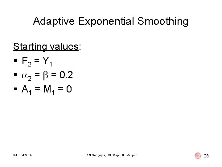
Adaptive Exponential Smoothing Starting values: § F 2 = Y 1 § 2 = = 0. 2 § A 1 = M 1 = 0 IME 634: MDA R. N. Sengupta, IME Dept. , IIT Kanpur 28

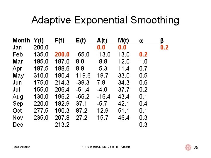
Adaptive Exponential Smoothing Month Jan Feb Mar Apr May Jun Jul Aug Sep Oct Nov Dec IME 634: MDA Y(t) 200. 0 135. 0 197. 5 310. 0 175. 0 155. 0 130. 0 220. 0 277. 5 235. 0 F(t) E(t) 200. 0 187. 0 188. 6 190. 4 214. 3 206. 4 196. 2 182. 9 190. 3 207. 8 213. 2 -65. 0 8. 9 119. 6 -39. 3 -51. 4 -66. 2 37. 1 87. 2 27. 2 A(t) 0. 0 -13. 0 -8. 8 -5. 3 19. 7 7. 9 -4. 0 -16. 4 -5. 7 12. 9 15. 7 M(t) 0. 0 13. 0 12. 0 11. 4 33. 0 34. 3 37. 7 43. 4 42. 1 51. 1 46. 4 R. N. Sengupta, IME Dept. , IIT Kanpur 0. 2 1. 0 0. 7 0. 5 0. 6 0. 2 0. 1 0. 4 0. 1 0. 3 29

Adaptive Exponential Smoothing IME 634: MDA R. N. Sengupta, IME Dept. , IIT Kanpur 30

Adaptive Exponential Smoothing IME 634: MDA R. N. Sengupta, IME Dept. , IIT Kanpur 31

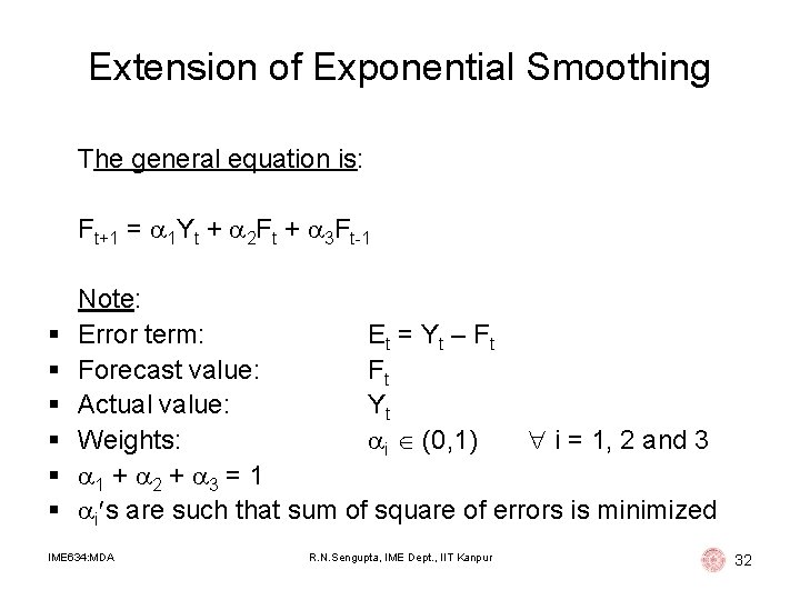
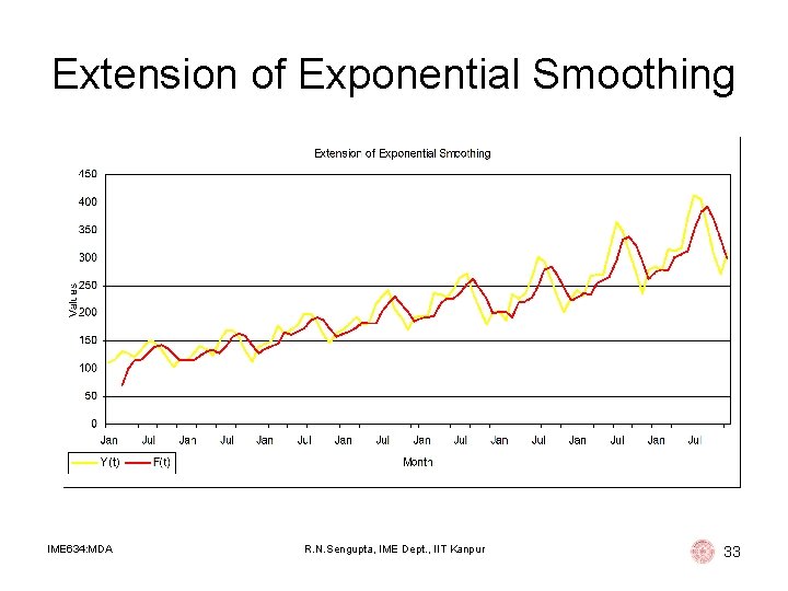
Extension of Exponential Smoothing The general equation is: Ft+1 = 1 Yt + 2 Ft + 3 Ft-1 § § § Note: Error term: Et = Y t – F t Forecast value: Ft Actual value: Yt Weights: i (0, 1) i = 1, 2 and 3 1 + 2 + 3 = 1 i s are such that sum of square of errors is minimized IME 634: MDA R. N. Sengupta, IME Dept. , IIT Kanpur 32

Extension of Exponential Smoothing IME 634: MDA R. N. Sengupta, IME Dept. , IIT Kanpur 33

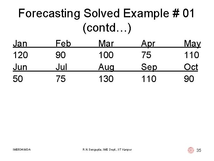
Forecasting Solved Example # 01 The IIT Home Tutor Solutions Pvt. Ltd. helps customers to find private tuitions and coaching centers in Kanpur city as well as online tutors. This supply business is competitive, and the ability to deliver talented as well-educated tutors promptly is a big factor in getting new customers and maintaining old ones. The manager of the company wants to be certain that enough tutors are available at hand to meet demand promptly. Therefore, the manager wants to be able to forecast the demand for requirement of tutors during the next month. From the records of previous orders, management has accumulated the following data for the past 10 months: IME 634: MDA R. N. Sengupta, IME Dept. , IIT Kanpur 34

Forecasting Solved Example # 01 (contd…) Jan 120 Jun 50 IME 634: MDA Feb 90 Jul 75 Mar 100 Aug 130 R. N. Sengupta, IME Dept. , IIT Kanpur Apr 75 Sep 110 May 110 Oct 90 35

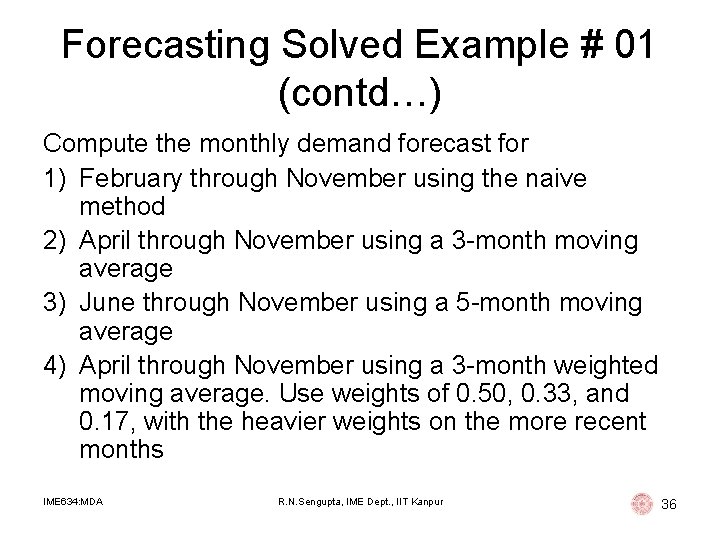
Forecasting Solved Example # 01 (contd…) Compute the monthly demand forecast for 1) February through November using the naive method 2) April through November using a 3 -month moving average 3) June through November using a 5 -month moving average 4) April through November using a 3 -month weighted moving average. Use weights of 0. 50, 0. 33, and 0. 17, with the heavier weights on the more recent months IME 634: MDA R. N. Sengupta, IME Dept. , IIT Kanpur 36

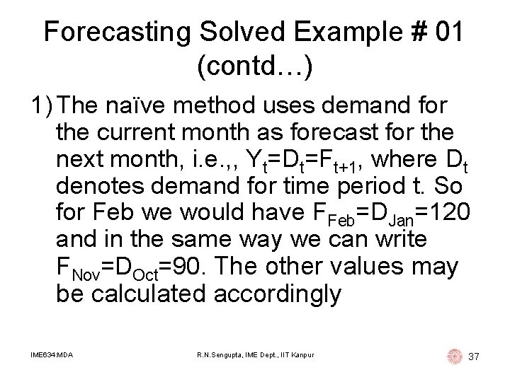
Forecasting Solved Example # 01 (contd…) 1) The naïve method uses demand for the current month as forecast for the next month, i. e. , , Yt=Dt=Ft+1, where Dt denotes demand for time period t. So for Feb we would have FFeb=DJan=120 and in the same way we can write FNov=DOct=90. The other values may be calculated accordingly IME 634: MDA R. N. Sengupta, IME Dept. , IIT Kanpur 37

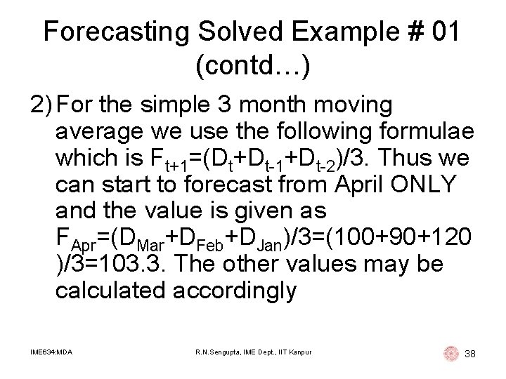
Forecasting Solved Example # 01 (contd…) 2) For the simple 3 month moving average we use the following formulae which is Ft+1=(Dt+Dt-1+Dt-2)/3. Thus we can start to forecast from April ONLY and the value is given as FApr=(DMar+DFeb+DJan)/3=(100+90+120 )/3=103. 3. The other values may be calculated accordingly IME 634: MDA R. N. Sengupta, IME Dept. , IIT Kanpur 38

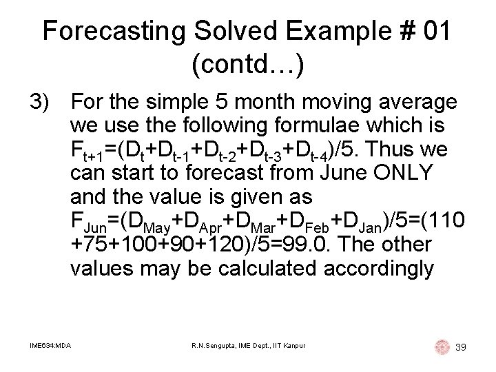
Forecasting Solved Example # 01 (contd…) 3) For the simple 5 month moving average we use the following formulae which is Ft+1=(Dt+Dt-1+Dt-2+Dt-3+Dt-4)/5. Thus we can start to forecast from June ONLY and the value is given as FJun=(DMay+DApr+DMar+DFeb+DJan)/5=(110 +75+100+90+120)/5=99. 0. The other values may be calculated accordingly IME 634: MDA R. N. Sengupta, IME Dept. , IIT Kanpur 39

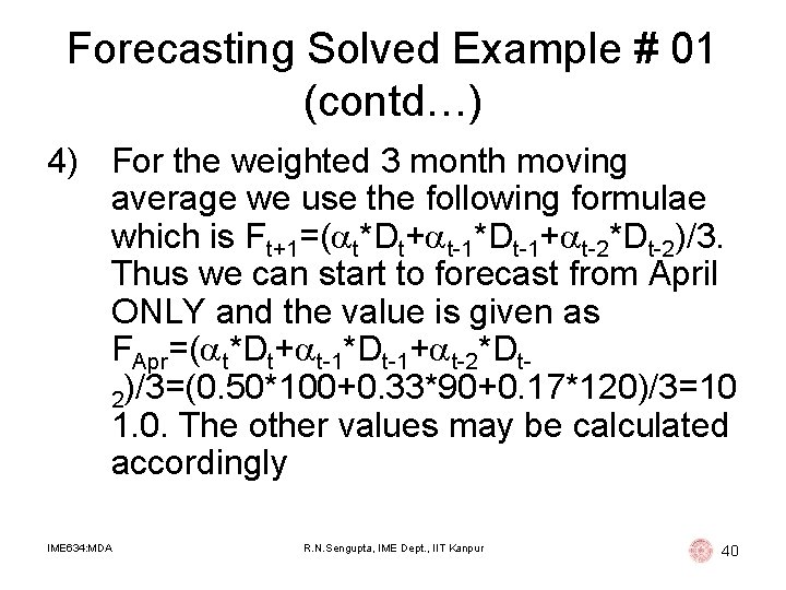
Forecasting Solved Example # 01 (contd…) 4) For the weighted 3 month moving average we use the following formulae which is Ft+1=( t*Dt+ t-1*Dt-1+ t-2*Dt-2)/3. Thus we can start to forecast from April ONLY and the value is given as FApr=( t*Dt+ t-1*Dt-1+ t-2*Dt 2)/3=(0. 50*100+0. 33*90+0. 17*120)/3=10 1. 0. The other values may be calculated accordingly IME 634: MDA R. N. Sengupta, IME Dept. , IIT Kanpur 40

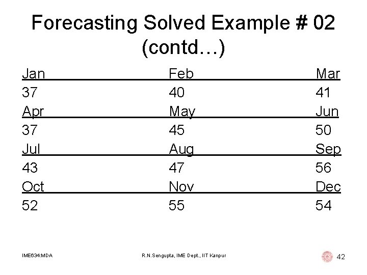
Forecasting Solved Example # 02 IIT Kanpur Furniture Ltd. makes customized furniture. Orders are received via online request and subsequently demand is fulfilled. Formed and operated by IIT Kanpur students, the company has had steady growth since it started. Due to volatility of demand, they need a good forecast of demand for their furniture so that they will know how much raw material to purchase and stock. They have compiled demand data for the last 12 months as reported below IME 634: MDA R. N. Sengupta, IME Dept. , IIT Kanpur 41

Forecasting Solved Example # 02 (contd…) Jan 37 Apr 37 Jul 43 Oct 52 IME 634: MDA Feb 40 May 45 Aug 47 Nov 55 R. N. Sengupta, IME Dept. , IIT Kanpur Mar 41 Jun 50 Sep 56 Dec 54 42

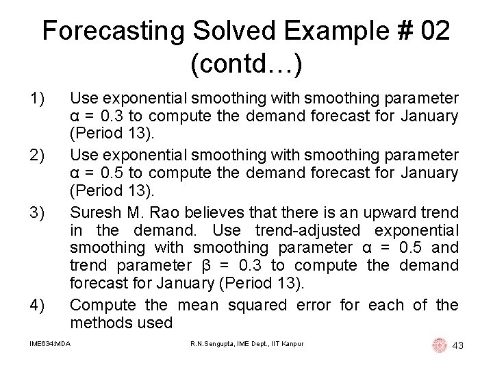
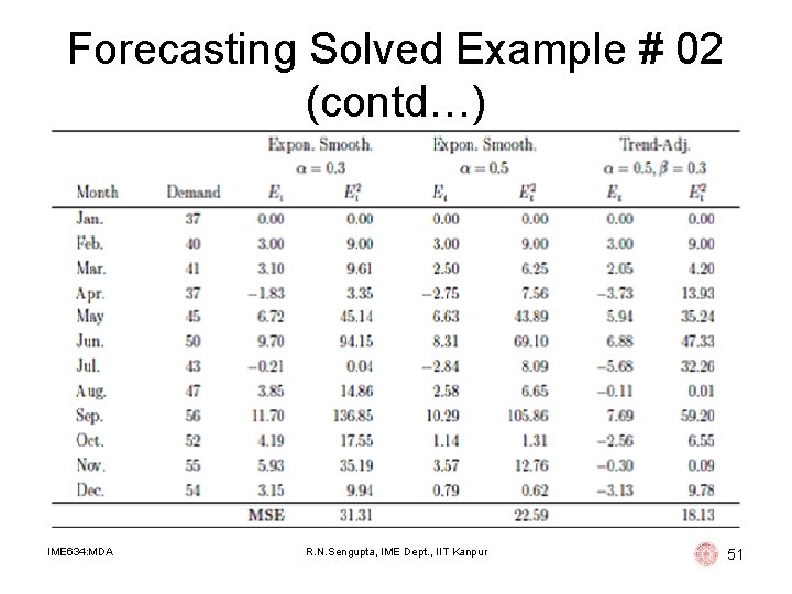
Forecasting Solved Example # 02 (contd…) 1) 2) 3) 4) Use exponential smoothing with smoothing parameter α = 0. 3 to compute the demand forecast for January (Period 13). Use exponential smoothing with smoothing parameter α = 0. 5 to compute the demand forecast for January (Period 13). Suresh M. Rao believes that there is an upward trend in the demand. Use trend-adjusted exponential smoothing with smoothing parameter α = 0. 5 and trend parameter β = 0. 3 to compute the demand forecast for January (Period 13). Compute the mean squared error for each of the methods used IME 634: MDA R. N. Sengupta, IME Dept. , IIT Kanpur 43

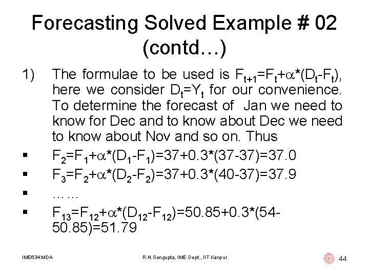
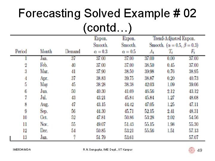
Forecasting Solved Example # 02 (contd…) 1) § § The formulae to be used is Ft+1=Ft+ *(Dt-Ft), here we consider Dt=Yt for our convenience. To determine the forecast of Jan we need to know for Dec and to know about Dec we need to know about Nov and so on. Thus F 2=F 1+ *(D 1 -F 1)=37+0. 3*(37 -37)=37. 0 F 3=F 2+ *(D 2 -F 2)=37+0. 3*(40 -37)=37. 9 …… F 13=F 12+ *(D 12 -F 12)=50. 85+0. 3*(5450. 85)=51. 79 IME 634: MDA R. N. Sengupta, IME Dept. , IIT Kanpur 44

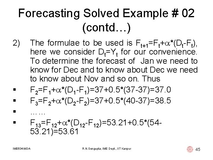
Forecasting Solved Example # 02 (contd…) 2) § § The formulae to be used is Ft+1=Ft+ *(Dt-Ft), here we consider Dt=Yt for our convenience. To determine the forecast of Jan we need to know for Dec and to know about Dec we need to know about Nov and so on. Thus F 2=F 1+ *(D 1 -F 1)=37+0. 5*(37 -37)=37. 0 F 3=F 2+ *(D 2 -F 2)=37+0. 5*(40 -37)=38. 5 …… F 13=F 12+ *(D 12 -F 12)=53. 21+0. 5*(5453. 21)=53. 61 IME 634: MDA R. N. Sengupta, IME Dept. , IIT Kanpur 45

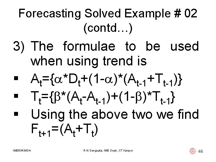
Forecasting Solved Example # 02 (contd…) 3) The formulae to be used when using trend is § At={ *Dt+(1 - )*(At-1+Tt-1)} § Tt={ *(At-At-1)+(1 - )*Tt-1} § Using the above two we find Ft+1=(At+Tt) IME 634: MDA R. N. Sengupta, IME Dept. , IIT Kanpur 46

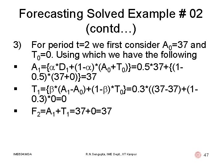
Forecasting Solved Example # 02 (contd…) 3) § § § For period t=2 we first consider A 0=37 and T 0=0. Using which we have the following A 1={ *D 1+(1 - )*(A 0+T 0)}=0. 5*37+{(10. 5)*(37+0)}=37 T 1={ *(A 1 -A 0)+(1 - )*T 0}=0. 3*((37 -37)+(10. 3)*0=0 F 2=A 1+T 1=37+0=37 IME 634: MDA R. N. Sengupta, IME Dept. , IIT Kanpur 47

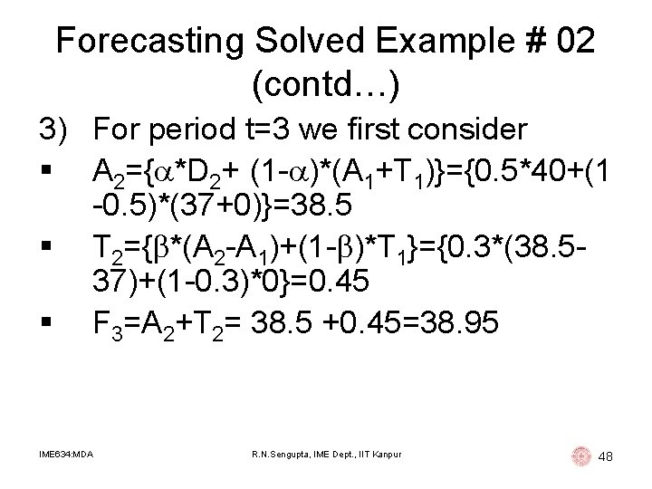
Forecasting Solved Example # 02 (contd…) 3) For period t=3 we first consider § A 2={ *D 2+ (1 - )*(A 1+T 1)}={0. 5*40+(1 -0. 5)*(37+0)}=38. 5 § T 2={ *(A 2 -A 1)+(1 - )*T 1}={0. 3*(38. 537)+(1 -0. 3)*0}=0. 45 § F 3=A 2+T 2= 38. 5 +0. 45=38. 95 IME 634: MDA R. N. Sengupta, IME Dept. , IIT Kanpur 48

Forecasting Solved Example # 02 (contd…) IME 634: MDA R. N. Sengupta, IME Dept. , IIT Kanpur 49

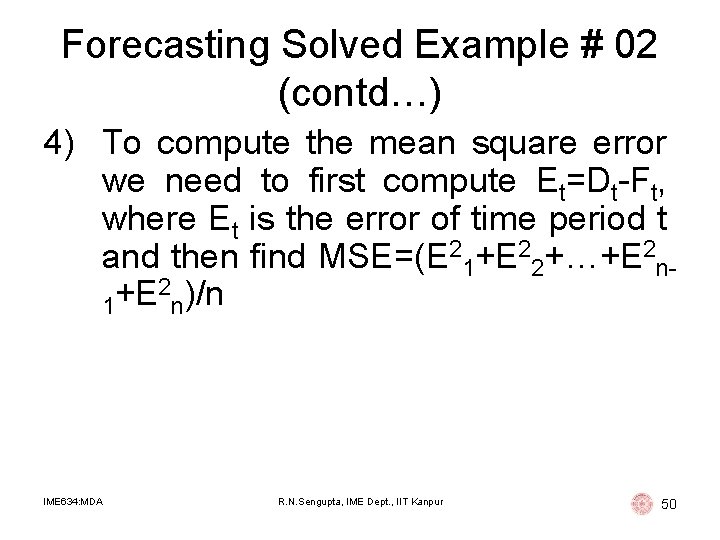
Forecasting Solved Example # 02 (contd…) 4) To compute the mean square error we need to first compute Et=Dt-Ft, where Et is the error of time period t and then find MSE=(E 21+E 22+…+E 2 n 2 )/n +E 1 n IME 634: MDA R. N. Sengupta, IME Dept. , IIT Kanpur 50

Forecasting Solved Example # 02 (contd…) IME 634: MDA R. N. Sengupta, IME Dept. , IIT Kanpur 51

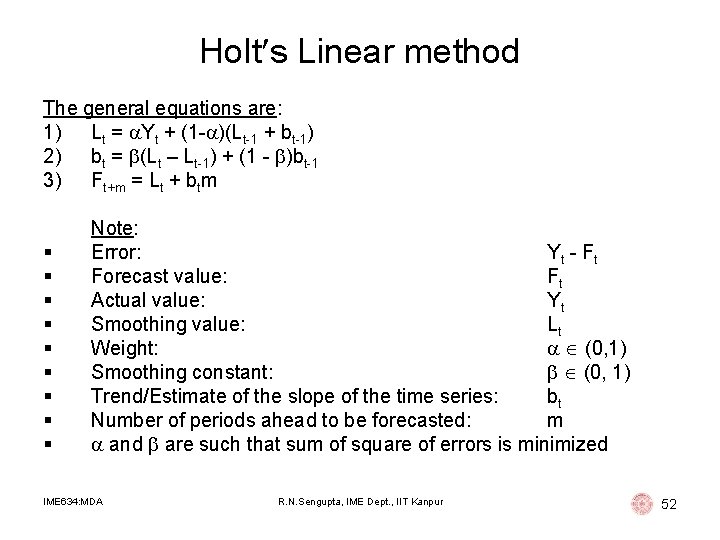
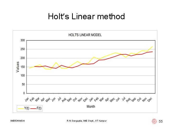
Holt s Linear method The general equations are: 1) Lt = Yt + (1 - )(Lt-1 + bt-1) 2) bt = (Lt – Lt-1) + (1 - )bt-1 3) Ft+m = Lt + btm § § § § § Note: Error: Yt - F t Forecast value: Ft Actual value: Yt Smoothing value: Lt Weight: (0, 1) Smoothing constant: (0, 1) Trend/Estimate of the slope of the time series: bt Number of periods ahead to be forecasted: m and are such that sum of square of errors is minimized IME 634: MDA R. N. Sengupta, IME Dept. , IIT Kanpur 52

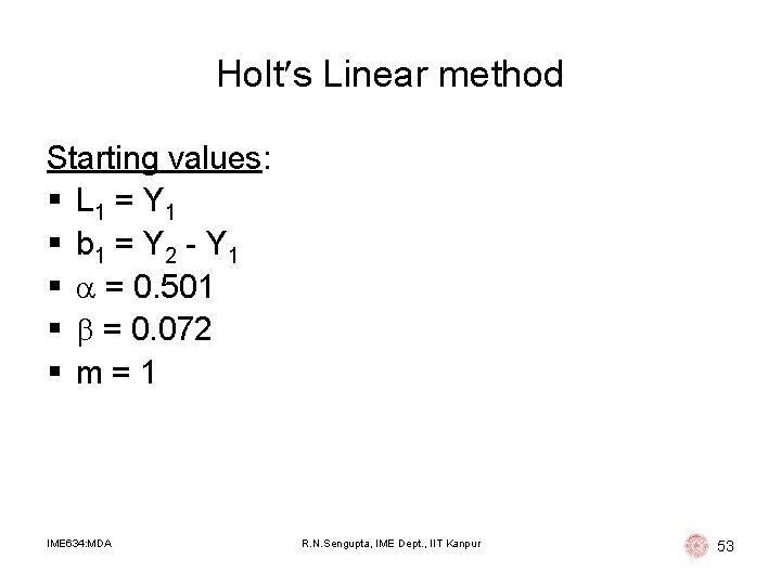
Holt s Linear method Starting values: § L 1 = Y 1 § b 1 = Y 2 - Y 1 § = 0. 501 § = 0. 072 § m=1 IME 634: MDA R. N. Sengupta, IME Dept. , IIT Kanpur 53

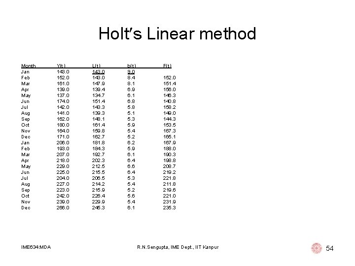
Holt s Linear method Month Jan Feb Mar Apr May Jun Jul Aug Sep Oct Nov Dec IME 634: MDA Y(t) 143. 0 152. 0 161. 0 139. 0 137. 0 174. 0 142. 0 141. 0 162. 0 180. 0 164. 0 171. 0 206. 0 193. 0 207. 0 218. 0 229. 0 225. 0 204. 0 227. 0 223. 0 242. 0 239. 0 266. 0 L(t) 143. 0 147. 9 139. 4 134. 7 151. 4 143. 3 139. 3 148. 1 161. 4 159. 8 162. 7 181. 8 184. 3 192. 7 202. 3 212. 5 215. 5 206. 5 214. 2 215. 9 226. 4 229. 9 245. 3 b(t) 9. 0 8. 4 8. 1 6. 9 6. 1 6. 8 5. 1 5. 3 5. 9 5. 4 5. 2 6. 2 5. 9 6. 1 6. 4 6. 6 6. 4 5. 3 5. 4 5. 2 5. 6 5. 4 6. 1 F(t) 152. 0 151. 4 156. 0 146. 3 140. 8 158. 2 149. 0 144. 3 153. 5 167. 3 165. 1 167. 9 188. 0 190. 3 198. 8 208. 7 219. 2 221. 8 219. 6 221. 0 231. 9 235. 3 R. N. Sengupta, IME Dept. , IIT Kanpur 54

Holt s Linear method IME 634: MDA R. N. Sengupta, IME Dept. , IIT Kanpur 55

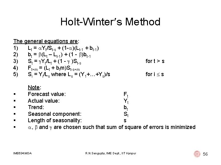
Holt-Winter s Method The general equations are: 1) Lt = Yt/St-s + (1 - )(Lt-1 + bt-1) 2) bt = (Lt – Lt-1) + (1 - )bt-1 3) St = Yt/Lt + (1 - )St-s 4) Ft+m = (Lt + btm)St-s+m 5) Si = Yi/Ls where Ls = (Y 1+…+Ys)/s § § § for t > s for i s Note: Forecast value: Ft Actual value: Yt Trend: bt Seasonal component: St Length of seasonality: s , and are chosen such that sum of square of errors is minimized IME 634: MDA R. N. Sengupta, IME Dept. , IIT Kanpur 56

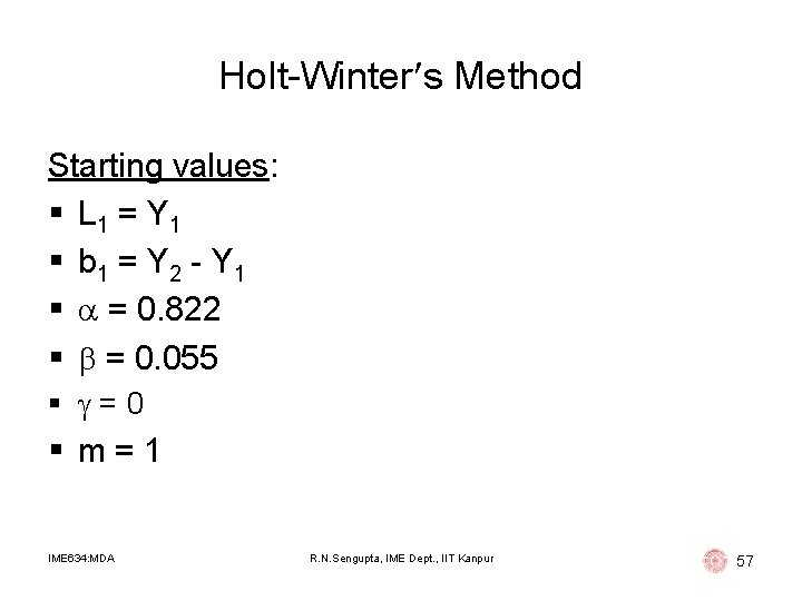
Holt-Winter s Method Starting values: § L 1 = Y 1 § b 1 = Y 2 - Y 1 § = 0. 822 § = 0. 055 § =0 § m=1 IME 634: MDA R. N. Sengupta, IME Dept. , IIT Kanpur 57

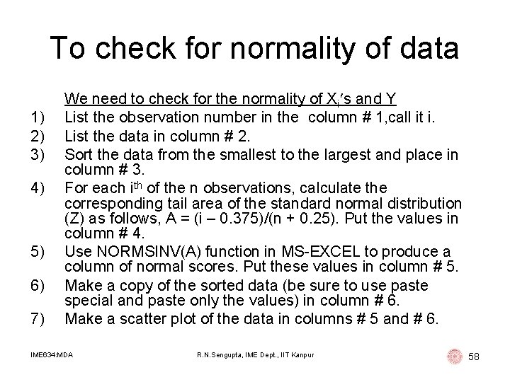
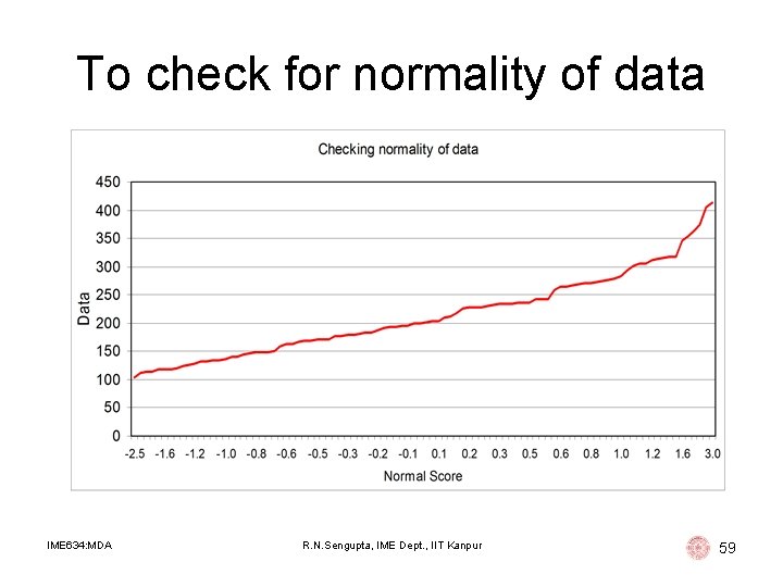
To check for normality of data 1) 2) 3) 4) 5) 6) 7) We need to check for the normality of Xi s and Y List the observation number in the column # 1, call it i. List the data in column # 2. Sort the data from the smallest to the largest and place in column # 3. For each ith of the n observations, calculate the corresponding tail area of the standard normal distribution (Z) as follows, A = (i – 0. 375)/(n + 0. 25). Put the values in column # 4. Use NORMSINV(A) function in MS-EXCEL to produce a column of normal scores. Put these values in column # 5. Make a copy of the sorted data (be sure to use paste special and paste only the values) in column # 6. Make a scatter plot of the data in columns # 5 and # 6. IME 634: MDA R. N. Sengupta, IME Dept. , IIT Kanpur 58

To check for normality of data IME 634: MDA R. N. Sengupta, IME Dept. , IIT Kanpur 59

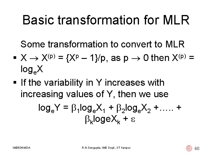
Basic transformation for MLR Some transformation to convert to MLR § X X(p) = {Xp – 1}/p, as p 0 then X(p) = loge. X § If the variability in Y increases with increasing values of Y, then we use loge. Y = 1 loge. X 1 + 2 loge. X 2 +…. . + kloge. Xk + IME 634: MDA R. N. Sengupta, IME Dept. , IIT Kanpur 60

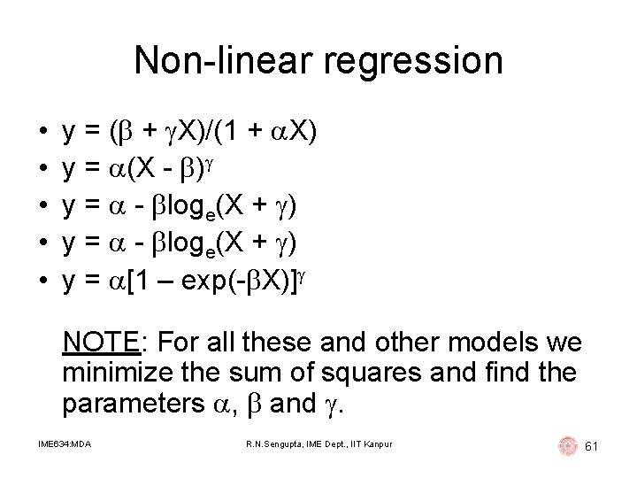
Non-linear regression • • • y = ( + X)/(1 + X) y = (X - ) y = - loge(X + ) y = [1 – exp(- X)] NOTE: For all these and other models we minimize the sum of squares and find the parameters , and . IME 634: MDA R. N. Sengupta, IME Dept. , IIT Kanpur 61