Decision Analysis Problem Formulation Decision Making without Probabilities

Decision Analysis Problem Formulation Decision Making without Probabilities Decision Making with Probabilities Risk Analysis and Sensitivity Analysis Decision Analysis with Sample Information Computing Branch Probabilities Utility and Decision Making Dr. C. Lightner Fayetteville State University 1

Problem Formulation A decision problem is characterized by decision alternatives, states of nature, and resulting payoffs. The decision alternatives are the different possible strategies the decision maker can employ. The states of nature refer to future events, not under the control of the decision maker, which will ultimately affect decision results. States of nature should be defined so that they are mutually exclusive and contain all possible future events that could affect the results of all potential decisions. Dr. C. Lightner Fayetteville State University 2

Decision Theory Models Decision theory problems are generally represented as one of the following: – Influence Diagram – Payoff Table – Decision Tree Dr. C. Lightner Fayetteville State University 3

Influence Diagrams An influence diagram is a graphical device showing the relationships among the decisions, the chance events, and the consequences. Squares or rectangles depict decision nodes. Circles or ovals depict chance nodes. Diamonds depict consequence nodes. Lines or arcs connecting the nodes show the direction of influence. Dr. C. Lightner Fayetteville State University 4

Payoff Tables The consequence resulting from a specific combination of a decision alternative and a state of nature is a payoff. A table showing payoffs for all combinations of decision alternatives and states of nature is a payoff table. Payoffs can be expressed in terms of profit, cost, time, distance or any other appropriate measure. Dr. C. Lightner Fayetteville State University 5

Decision Trees A decision tree is a chronological representation of the decision problem. Each decision tree has two types of nodes; round nodes correspond to the states of nature while square nodes correspond to the decision alternatives. The branches leaving each round node represent the different states of nature while the branches leaving each square node represent the different decision alternatives. At the end of each limb of a tree are the payoffs attained from the series of branches making up that limb. Dr. C. Lightner Fayetteville State University 6

Example: CAL Condominium Complex A developer must decide how large a luxury condominium complex to build – small, medium, or large. The profitability of this complex depends upon the future level of demand for the complex’s condominiums. Dr. C. Lightner Fayetteville State University 7

CAL Condos: Elements of Decision Theory States of nature: The states of nature could be defined as low demand high demand. Alternatives: CAL could decide to build a small, medium, or large condominium complex. Payoffs: The profit for each alternative under each potential state of nature is going to be determined. We develop different models for this problem on the following slides. Dr. C. Lightner Fayetteville State University 8

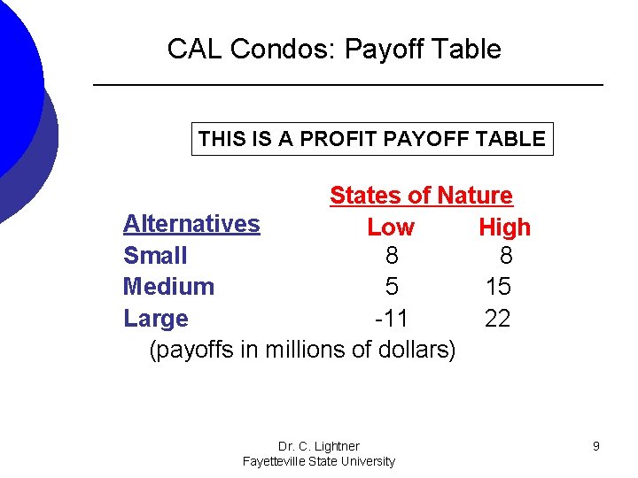
CAL Condos: Payoff Table THIS IS A PROFIT PAYOFF TABLE States of Nature Alternatives Low High Small 8 8 Medium 5 15 Large -11 22 (payoffs in millions of dollars) Dr. C. Lightner Fayetteville State University 9

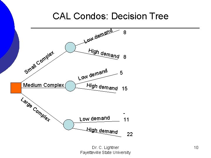
CAL Condos: Decision Tree Low all Sm m o C rg e 8 eman d 8 High d x e l p nd ma e d w 5 Lo Medium Complex La nd a dem High dem and 15 Co m ple x Low demand High demand 11 22 Dr. C. Lightner Fayetteville State University 10

Decision Making without Probabilities Three commonly used criteria for decision making when probability information regarding the likelihood of the states of nature is unavailable are: – the optimistic approach – the conservative approach – the minimax regret approach. Dr. C. Lightner Fayetteville State University 11

Optimistic Approach The optimistic approach would be used by an optimistic decision maker. The decision with the best possible payoff is chosen. If the payoff table was in terms of costs, the decision with the lowest cost would be chosen. If the payoff table was in terms of profits, the decision with the highest profit would be chosen. Dr. C. Lightner Fayetteville State University 12

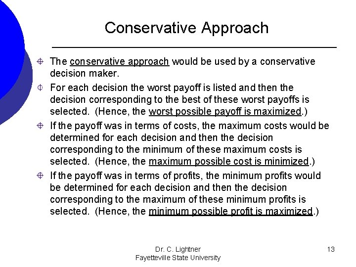
Conservative Approach The conservative approach would be used by a conservative decision maker. For each decision the worst payoff is listed and then the decision corresponding to the best of these worst payoffs is selected. (Hence, the worst possible payoff is maximized. ) If the payoff was in terms of costs, the maximum costs would be determined for each decision and then the decision corresponding to the minimum of these maximum costs is selected. (Hence, the maximum possible cost is minimized. ) If the payoff was in terms of profits, the minimum profits would be determined for each decision and then the decision corresponding to the maximum of these minimum profits is selected. (Hence, the minimum possible profit is maximized. ) Dr. C. Lightner Fayetteville State University 13

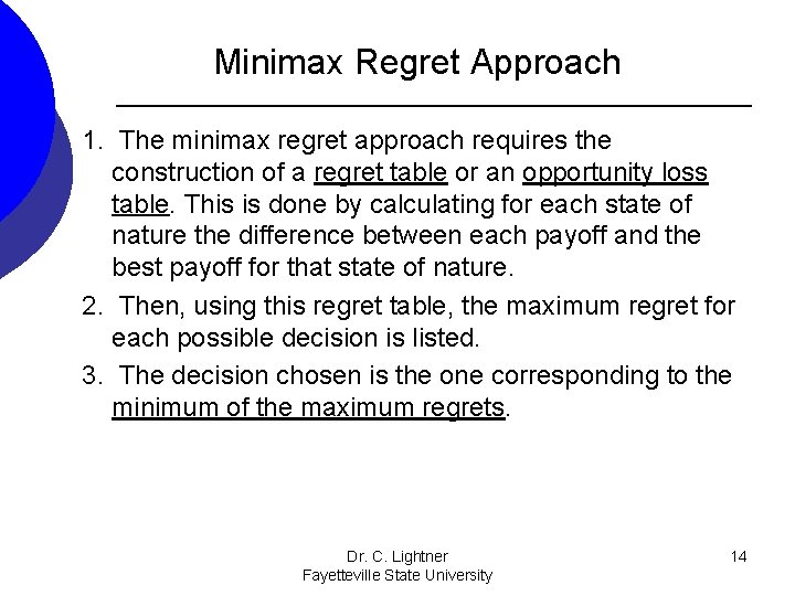
Minimax Regret Approach 1. The minimax regret approach requires the construction of a regret table or an opportunity loss table. This is done by calculating for each state of nature the difference between each payoff and the best payoff for that state of nature. 2. Then, using this regret table, the maximum regret for each possible decision is listed. 3. The decision chosen is the one corresponding to the minimum of the maximum regrets. Dr. C. Lightner Fayetteville State University 14

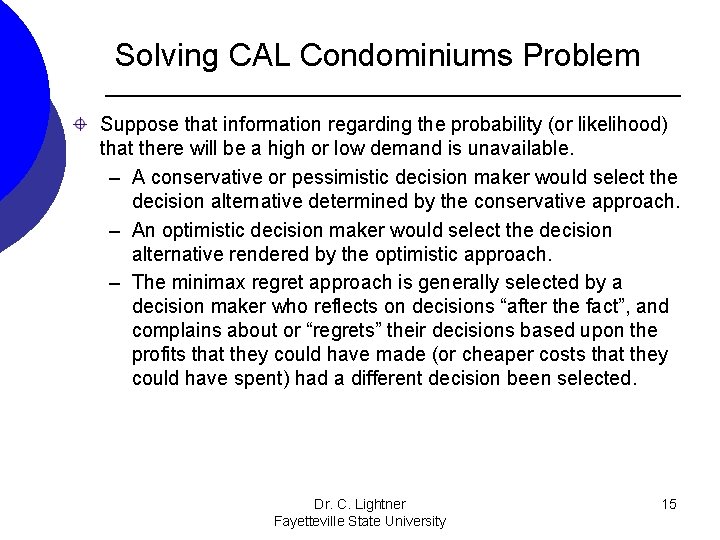
Solving CAL Condominiums Problem Suppose that information regarding the probability (or likelihood) that there will be a high or low demand is unavailable. – A conservative or pessimistic decision maker would select the decision alternative determined by the conservative approach. – An optimistic decision maker would select the decision alternative rendered by the optimistic approach. – The minimax regret approach is generally selected by a decision maker who reflects on decisions “after the fact”, and complains about or “regrets” their decisions based upon the profits that they could have made (or cheaper costs that they could have spent) had a different decision been selected. Dr. C. Lightner Fayetteville State University 15

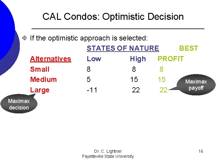
CAL Condos: Optimistic Decision If the optimistic approach is selected: STATES OF NATURE BEST Alternatives Low High PROFIT Small 8 8 8 Medium 5 15 15 Maximax payoff Large -11 22 22 Maximax decision Dr. C. Lightner Fayetteville State University 16

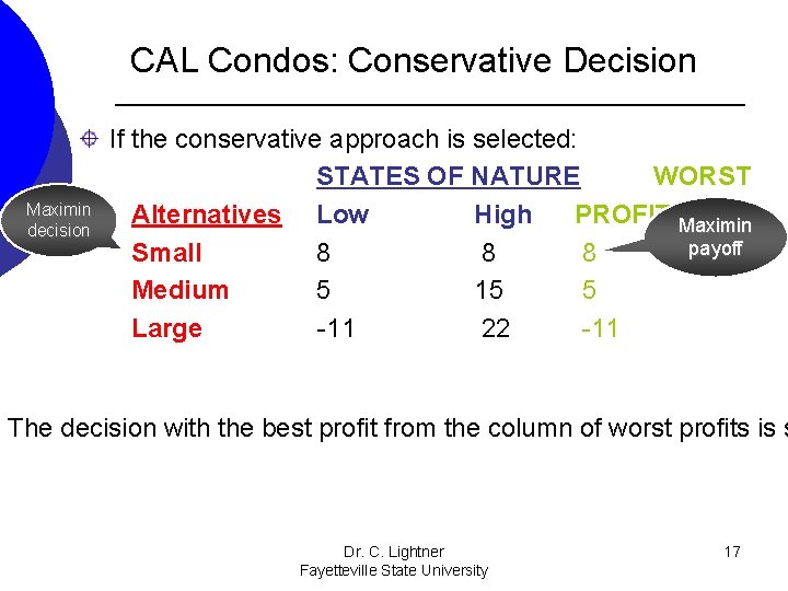
CAL Condos: Conservative Decision Maximin decision If the conservative approach is selected: STATES OF NATURE WORST Alternatives Low High PROFIT Maximin payoff Small 8 8 8 Medium 5 15 5 Large -11 22 -11 The decision with the best profit from the column of worst profits is s Dr. C. Lightner Fayetteville State University 17

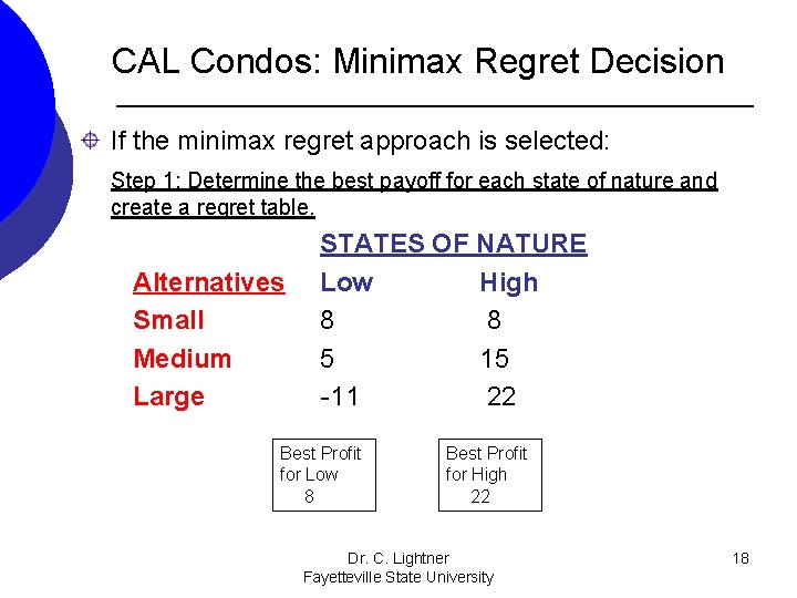
CAL Condos: Minimax Regret Decision If the minimax regret approach is selected: Step 1: Determine the best payoff for each state of nature and create a regret table. Alternatives Small Medium Large STATES OF NATURE Low High 8 8 5 15 -11 22 Best Profit for Low 8 Best Profit for High 22 Dr. C. Lightner Fayetteville State University 18

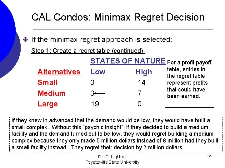
CAL Condos: Minimax Regret Decision If the minimax regret approach is selected: Step 1: Create a regret table (continued). Alternatives Small Medium Large STATES OF NATURE For a profit payoff table, entries in Low High the regret table represent profits 0 14 that could have 3 7 been earned. 19 0 If they knew in advanced that the demand would be low, they would have built a small complex. Without this “psychic insight”, if they decided to build a medium facility and the demand turned out to be low, they would regret building a medium complex because they only made 5 million dollars instead of 8 million had they built a small facility instead. They regret their decision by 3 million dollars. Dr. C. Lightner Fayetteville State University 19

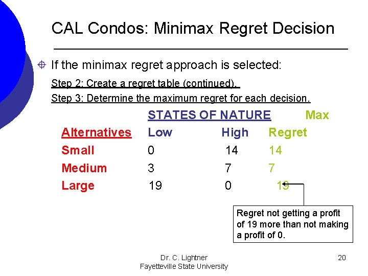
CAL Condos: Minimax Regret Decision If the minimax regret approach is selected: Step 2: Create a regret table (continued). Step 3: Determine the maximum regret for each decision. Alternatives Small Medium Large STATES OF NATURE Max Low High Regret 0 14 14 3 7 7 19 0 19 Regret not getting a profit of 19 more than not making a profit of 0. Dr. C. Lightner Fayetteville State University 20

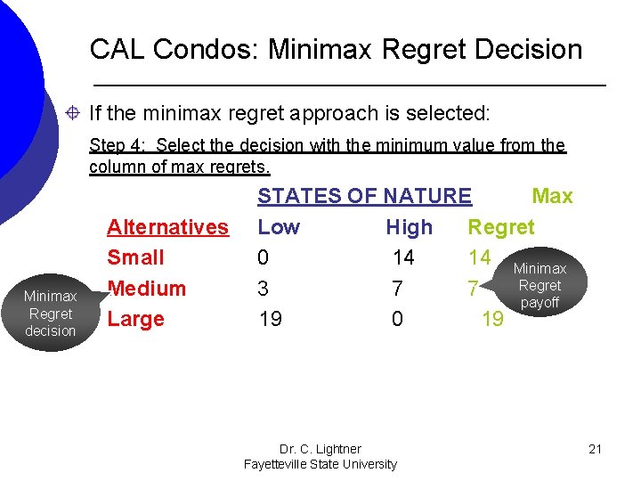
CAL Condos: Minimax Regret Decision If the minimax regret approach is selected: Step 4: Select the decision with the minimum value from the column of max regrets. Minimax Regret decision Alternatives Small Medium Large STATES OF NATURE Max Low High Regret 0 14 14 Minimax Regret 3 7 7 payoff 19 0 19 Dr. C. Lightner Fayetteville State University 21

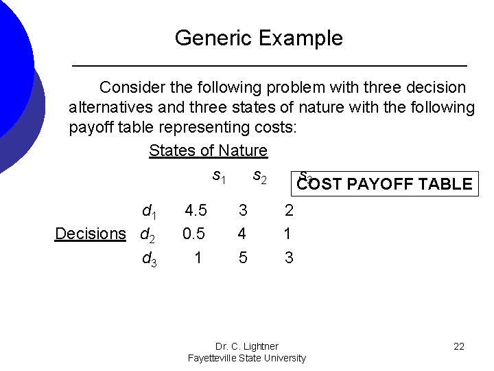
Generic Example Consider the following problem with three decision alternatives and three states of nature with the following payoff table representing costs: States of Nature s 1 s 2 s 3 COST PAYOFF TABLE d 1 Decisions d 2 d 3 4. 5 0. 5 1 3 4 5 2 1 3 Dr. C. Lightner Fayetteville State University 22

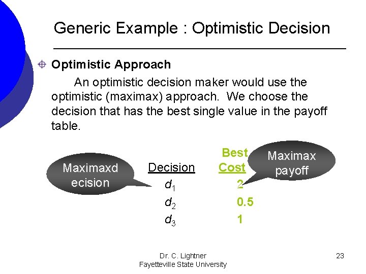
Generic Example : Optimistic Decision Optimistic Approach An optimistic decision maker would use the optimistic (maximax) approach. We choose the decision that has the best single value in the payoff table. Maximaxd ecision Decision d 1 d 2 d 3 Best Cost 2 0. 5 1 Dr. C. Lightner Fayetteville State University Maximax payoff 23

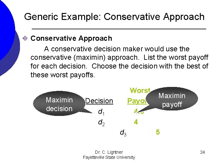
Generic Example: Conservative Approach A conservative decision maker would use the conservative (maximin) approach. List the worst payoff for each decision. Choose the decision with the best of these worst payoffs. Maximin decision Worst Payoff 4. 5 4 Decision d 1 d 2 d 3 Dr. C. Lightner Fayetteville State University Maximin payoff 5 24

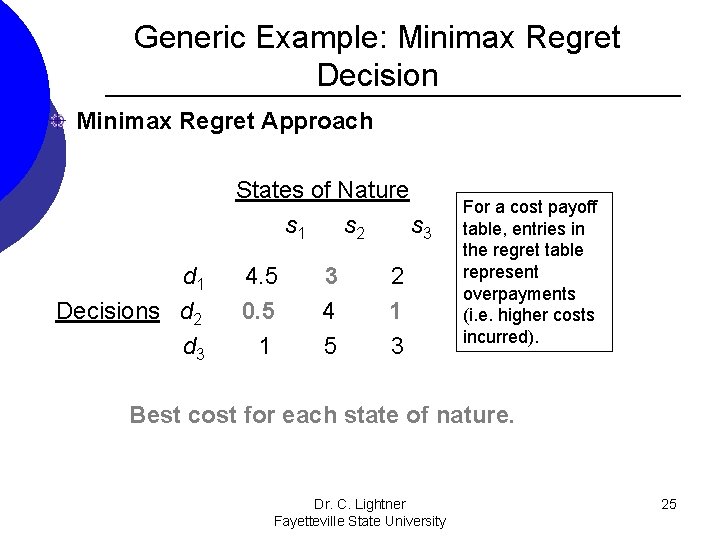
Generic Example: Minimax Regret Decision Minimax Regret Approach States of Nature s 1 s 2 s 3 d 1 Decisions d 2 d 3 4. 5 0. 5 1 3 4 5 2 1 3 For a cost payoff table, entries in the regret table represent overpayments (i. e. higher costs incurred). Best cost for each state of nature. Dr. C. Lightner Fayetteville State University 25

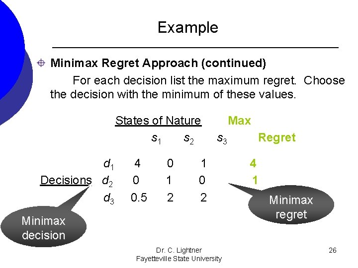
Example Minimax Regret Approach (continued) For each decision list the maximum regret. Choose the decision with the minimum of these values. States of Nature s 1 s 2 d 1 Decisions d 2 d 3 4 0 0. 5 0 1 2 Max s 3 1 0 2 Minimax decision Dr. C. Lightner Fayetteville State University Regret 4 1 2 Minimax regret 26

Decision Making with Probabilities Expected Value Approach – If probabilistic information regarding the states of nature is available, one may use the expected value (EV) approach. – Here the expected return for each decision is calculated by summing the products of the payoff under each state of nature and the probability of the respective state of nature occurring. – The decision yielding the best expected return is chosen. Dr. C. Lightner Fayetteville State University 27

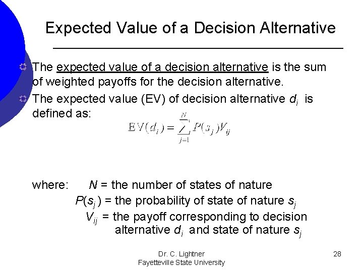
Expected Value of a Decision Alternative The expected value of a decision alternative is the sum of weighted payoffs for the decision alternative. The expected value (EV) of decision alternative di is defined as: where: N = the number of states of nature P(sj ) = the probability of state of nature sj Vij = the payoff corresponding to decision alternative di and state of nature sj Dr. C. Lightner Fayetteville State University 28

Example: Burger Prince Restaurant is contemplating opening a new restaurant on Main Street. It has three different models, each with a different seating capacity. Burger Prince estimates that the average number of customers per hour will be 80, 100, or 120. The payoff table (profits) for the three models is on the next slide. Dr. C. Lightner Fayetteville State University 29

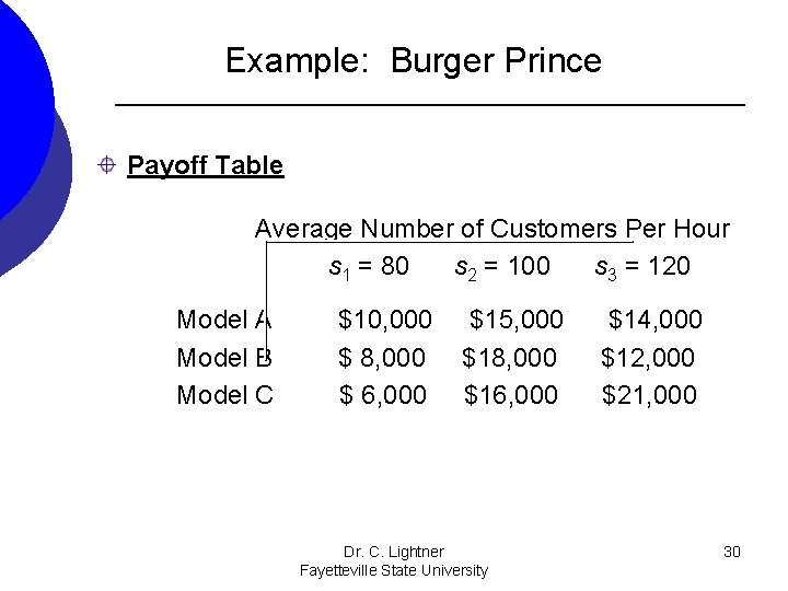
Example: Burger Prince Payoff Table Average Number of Customers Per Hour s 1 = 80 s 2 = 100 s 3 = 120 Model A Model B Model C $10, 000 $ 8, 000 $ 6, 000 $15, 000 $18, 000 $16, 000 Dr. C. Lightner Fayetteville State University $14, 000 $12, 000 $21, 000 30

Example: Burger Prince Expected Value Approach Calculate the expected value for each decision. The decision tree on the next slide can assist in this calculation. Here d 1, d 2, d 3 represent the decision alternatives of models A, B, C, and s 1, s 2, s 3 represent the states of nature of 80, 100, and 120. Dr. C. Lightner Fayetteville State University 31

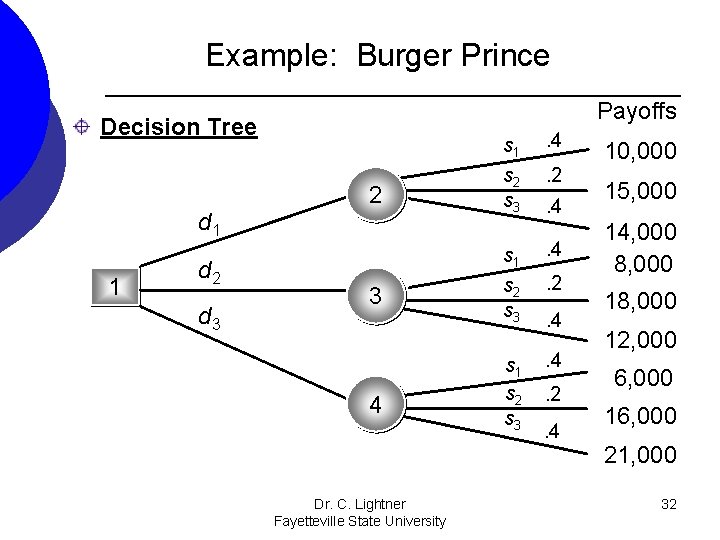
Example: Burger Prince Payoffs Decision Tree 2 d 1 1 d 2 d 3 3 4 Dr. C. Lightner Fayetteville State University s 1 s 2 s 3 . 4. 2. 4 s 1 . 4 s 2 s 3 . 2 s 1 s 2 s 3 . 4. 4. 2. 4 10, 000 15, 000 14, 000 8, 000 12, 000 6, 000 16, 000 21, 000 32

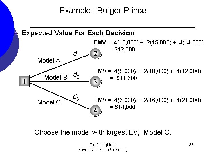
Example: Burger Prince Expected Value For Each Decision Model A 1 d 1 Model B d 2 Model C d 3 EMV =. 4(10, 000) +. 2(15, 000) +. 4(14, 000) = $12, 600 2 EMV =. 4(8, 000) +. 2(18, 000) +. 4(12, 000) = $11, 600 3 EMV =. 4(6, 000) +. 2(16, 000) +. 4(21, 000) = $14, 000 4 Choose the model with largest EV, Model C. Dr. C. Lightner Fayetteville State University 33

CAL Condos Revisited Suppose market research was conducted in the community where the complex will be built. This research allowed the company to estimate that the probability of low demand will be 0. 35, and the probability of high demand will be 0. 65. Which decision alternative should they select. Dr. C. Lightner Fayetteville State University 34

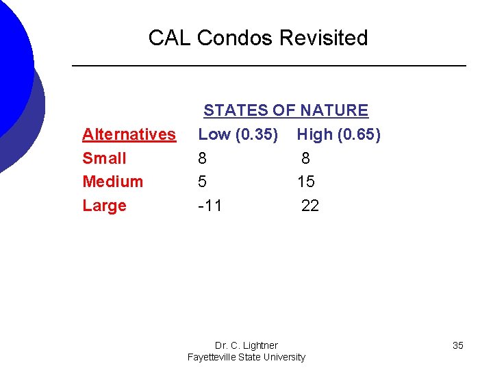
CAL Condos Revisited Alternatives Small Medium Large STATES OF NATURE Low (0. 35) High (0. 65) 8 8 5 15 -11 22 Dr. C. Lightner Fayetteville State University 35

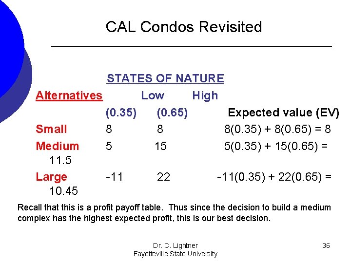
CAL Condos Revisited STATES OF NATURE Alternatives Low High (0. 35) (0. 65) Expected value (EV) Small 8 8 8(0. 35) + 8(0. 65) = 8 Medium 5 15 5(0. 35) + 15(0. 65) = 11. 5 Large -11 22 -11(0. 35) + 22(0. 65) = 10. 45 Recall that this is a profit payoff table. Thus since the decision to build a medium complex has the highest expected profit, this is our best decision. Dr. C. Lightner Fayetteville State University 36

Expected Value of Perfect Information Frequently information is available which can improve the probability estimates for the states of nature. The expected value of perfect information (EVPI) is the increase in the expected profit that would result if one knew with certainty which state of nature would occur. The EVPI provides an upper bound on the expected value of any sample or survey information. Dr. C. Lightner Fayetteville State University 37

Expected Value of Perfect Information EVPI Calculation – Step 1: Determine the optimal return corresponding to each state of nature. – Step 2: Compute the expected value of these optimal returns. – Step 3: Subtract the EV of the optimal decision from the amount determined in step (2). Dr. C. Lightner Fayetteville State University 38

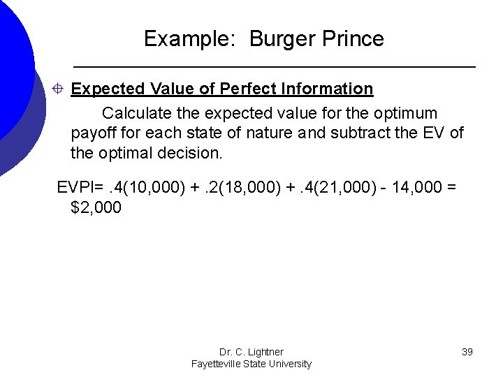
Example: Burger Prince Expected Value of Perfect Information Calculate the expected value for the optimum payoff for each state of nature and subtract the EV of the optimal decision. EVPI=. 4(10, 000) +. 2(18, 000) +. 4(21, 000) - 14, 000 = $2, 000 Dr. C. Lightner Fayetteville State University 39

Sensitivity Analysis Some of the quantities in a decision analysis, particularly the probabilities, are often intelligent guesses at best. It is important to accompany decision analysis with a sensitivity analysis. Sensitivity analysis can be used to determine how changes to the following inputs affect the recommended decision alternative: – probabilities for the states of nature – values of the payoffs If a small change in the value of one of the inputs causes a change in the recommended decision alternative, extra effort and care should be taken in estimating the input Dr. value. C. Lightner 40 Fayetteville State University

Sensitivity Analysis One approach to sensitivity analysis is to arbitrarily assign different values to the probabilities of the states of nature and/or the payoffs and resolve the problem. If the recommended decision changes, then you know that the solution is sensitive to the changes. For the special case of two states of nature, a graphical technique can be used to determine how sensitive the solution is to the probabilities associated with the states of nature. Dr. C. Lightner Fayetteville State University 41

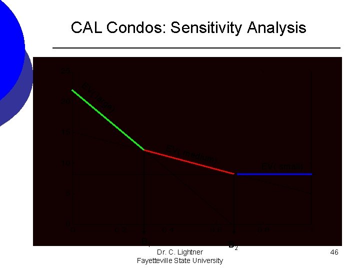
CAL Condos: Sensitivity Analysis This problem has two states of nature. Previously, we stated that CAL Condominiums estimated that the probability of future low demand is 0. 35 and 0. 65 is the probability of high demand. These probabilities yielded the recommended decision to build the medium complex. In order to see how sensitive this recommendation is to changing probability values, we will let p equal the probability of low demand. Thus (1 -p) is the probability of high demand. Therefore EV( small) = 8*p + 8*(1 -p)= 8 EV( medium) = 5*p + 15*(1 -p) = 15 – 10 p EV( large) = -11*p + Dr. 22*(1 -p) C. Lightner = 22 – 33 p 42 Fayetteville State University

CAL Condos: Sensitivity Analysis Next we will plot the expected value lines for each decision by plotting p on the x axis and EV on the y axis. EV( small) = 8 EV( medium) = 15 – 10 p EV( large) = 22 – 33 p Dr. C. Lightner Fayetteville State University 43

CAL Condos: Sensitivity Analysis EV ( la rg e) EV( m EV( small) edium ) Dr. C. Lightner Fayetteville State University 44

CAL Condos: Sensitivity Analysis Since CAL condominiums list payoffs are in terms of profits, we know that the highest profits is desirable. Look over the entire range of p (p=0 to p=1) and determine the range over which each decision yields the highest profits. Dr. C. Lightner Fayetteville State University 45

CAL Condos: Sensitivity Analysis EV ( la rg e) EV( m edium ) B 1 Dr. C. Lightner Fayetteville State University EV( small) B 2 46

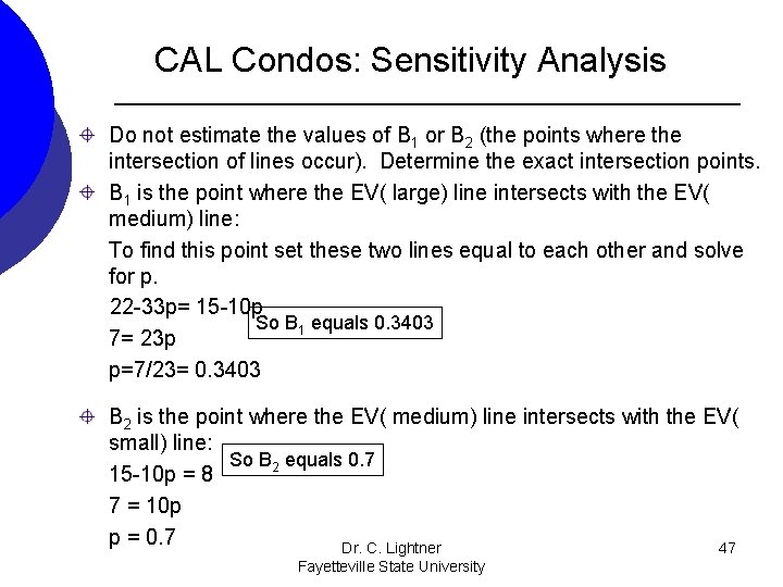
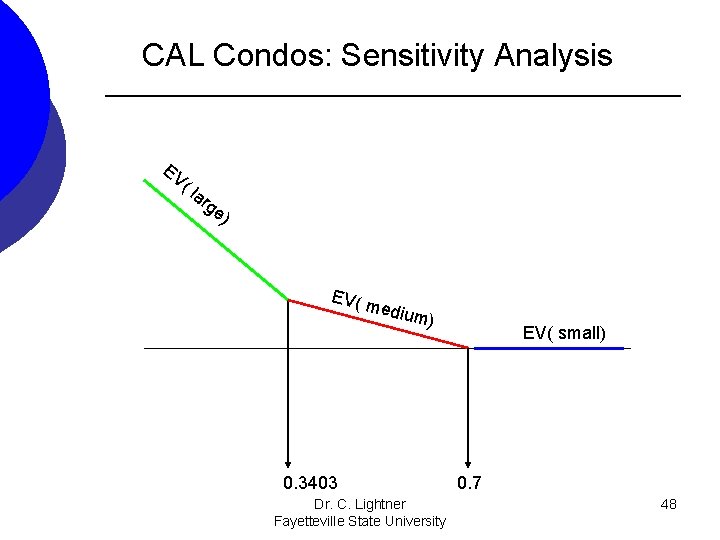
CAL Condos: Sensitivity Analysis Do not estimate the values of B 1 or B 2 (the points where the intersection of lines occur). Determine the exact intersection points. B 1 is the point where the EV( large) line intersects with the EV( medium) line: To find this point set these two lines equal to each other and solve for p. 22 -33 p= 15 -10 p So B 1 equals 0. 3403 7= 23 p p=7/23= 0. 3403 B 2 is the point where the EV( medium) line intersects with the EV( small) line: So B 2 equals 0. 7 15 -10 p = 8 7 = 10 p p = 0. 7 Dr. C. Lightner 47 Fayetteville State University

CAL Condos: Sensitivity Analysis EV ( la rg e) EV( m edium ) 0. 3403 Dr. C. Lightner Fayetteville State University EV( small) 0. 7 48

CAL Condos: Sensitivity Analysis From the graph we see that if the probability of low demand (p) is between 0 and 0. 3403, we recommend building a large complex. From the graph we see that if the probability of low demand (p) is between 0. 3403 and 0. 7, we recommend building a medium complex. From the graph we see that if the probability of low demand (p) is between 0. 7 and 1, we recommend building a large complex. From this sensitivity analysis we see that if CAL Condos estimate of 0. 35 for the probability of low demand was slightly lower, the recommended decision would change. Dr. C. Lightner 49 Fayetteville State University

End of Chapter 14 See your textbook for more examples and detailed explanations of all topics discussed in these notes. Dr. C. Lightner Fayetteville State University 50