ICBM Curso Electivo TericoPrctico Anlisis Cuantitativo de Colocalizacin

ICBM | Curso Electivo Teórico-Práctico | Análisis Cuantitativo de Colocalización en Microscopía Confocal 10 -17 |08|2007 Steffen Härtel Programa de Anatomía y Biología del Desarollo, Instituto de Ciencias Biomédicas, Facultad de Medicina, Universidad de Chile, Santiago, Chile

|-> Seminarios |-> Rodrigo Castillo: viernes, 10. 08. 07 @ 9. 30 -13. 00 Measurement of colocalization of objects in dual-color confocal images Manders E. (1993) Journal of Microscopy 169: 375 -382 |-> Ivan Alfarro: lunes, 13. 08. 07 @ 15 -18. 30 STED-Microscopy: Concepts for nanoscale resolution in fluorescence microscopy Hell S. , Dyba, M. , Jakobs S (2004) Current Opinion in Neurobiology 4: 599 -609 |-> Valentina Parra: lunes, 13. 08. 07 @ 15 -18. 30 Automatic and Quantitative Measurement of Protein-Protein Colocalization in Live Cells Costes et al. 2004 Biophys. J. 86, 3993– 4003 |-> Ariel Contreras: martes, 14. 08. 07 @ 9. 30 -13. 00 A syntaxin 1, Galphao, and N-type calcium channel complex at a presynaptic nerve terminal: analysis by quantitative immunocolocalization Li, Q. , Lau, A. , Morris, T. J. , Guo, L. , Fordyce, C. B. & Stanley, E. F. (2004) J. Neurosci. 24, 4070– 4081 |-> Barbra Toro: jueves, 16. 08. 07 @ 9. 30 -13. 00 Co-localization analysis of complex formation among membrane proteins by computerized fluorescence microscopy: application to immunofluorescence co-patching studies Lachmanovich, E. , Shvartsman, D. E. , Malka, Y. , Botvin, C. , Henis, Y. I. & Weiss, A. M. (2003) Journal of Microscopy. 212, 122– 131 |-> Nancy Leal: jueves, 16. 08. 07 @ 9. 30 -13. 00 Partial colocalization of glucocorticoid and mineralocorticoid receptors in discrete compartments in nuclei of rat hippocampus neurons Van Steensel, B. , van Binnendijk, E. , Hornsby, C. , van der Voort, H. , Krozowski, Z. , de Kloet, E. & van Driel, R. (1996) J. Cell Sci. 109, 787– 792 |-> Ximena Verges: viernes, 17. 08. 07 @ 9. 30 -13. 00 Multicolour analysis and local image correlation in confocal microscopy Demandolx, D. & Davoust, J. (1997) Journal of Microscopy 185, 21– 36 |-> Leonel Muñoz: viernes, 17. 08. 07 @ 9. 30 -13. 00 A guided tour into subcellular colocalization analysis in light microscopy Bolte S. & Cordelieres P. (2006) Journal of Microscopy, 224 (3): 213– 232
 defined by the Point Spread Function must be")
I|-> Intensity The observation volume (femtoliter) defined by the Point Spread Function must be considered as a mini-sprectrofluorimeter. Consider the Offset I(0) in order to calibrate your signal I(0) 0 ! Never saturate the signal: I Imax (255 for 8 bit) ! I > Imax I(0) > 0

II|-> Refractive index Use the right inmersion setup ! n 1 = n 2 ! Keep refractive index / index of refraction constant !
 is a function of the observation")
III|-> Nyquist The sampling frequency (or sampling distance) is a function of the observation volume (femtoliter) defined by the Point Spread Function (PSF): Consider sampling distances in x and y 50 nm and z 150 -300 nm for later deconvolution, or calculate the explicit sample distances directly. http: //support. svi. nl/wiki/Nyquist. Calculator

|-> what‘s up I. Image Adquisition I. a|-> Fundamentos de la microscopía confocal I. b|-> Fundamentos de la fluorescencia II. Deconvolution III. Segmentation IV. Analisys

|-> Fluorescencia Luminescencia: Interacciones. . . - Fluorescencia t ~ 10 -8 s - Fosforescencia t ~ 10 -3 -100 s producen cambios. . . Absorción / Excitación • intra- e inter moleculares. . . • espectrales • tiempos de vida • polarización • intensidad. . . t Emissión

|-> Jablonski Diagram Transiciones: con radiación sin radiación | Niveles: -> calor vibracionales electrónicos -> transferencia de energía (FRET) -> radicales. . . STED 10 -12 s Conversión interna 10 -8 s Intercombinación z 10 -6 - 1 s x/y 10 -15 s Absorción 10 -9 -10 -8 s Fluorescencia 10 -6 - 1 s Fosforescencia

|-> Franck Condon Frank Condon : ENERGY ‘Transiciones entre niveles electrónicos ocurren mucho mas rápido que movimientos de núcleos moleculares. ‘ (masaelectron / masaatom: 1 : 2000) -> Mirror Image Rule Stokes (Shift) : ‘La energía de emisión es menor a la energía de excitación. ‘ Distance [r]

|-> Mirror Image Rule

|-> Polarisación Polarización Anisotropía • a. MAX = 0, 39 • III~cos ² • a( ) (a) a: DPH. b: TMA-DPH, c: Carboxyl –DPH. Momentos dipolares µ de absorción y emission son parallelos. , viscosidad
 Resonance Energy Transfer: (F)RET Molecule 1 (DONOR) Molecule 2 (ACCEPTOR) Energy")
|-> FRET (Fluorescence) Resonance Energy Transfer: (F)RET Molecule 1 (DONOR) Molecule 2 (ACCEPTOR) Energy Transfer Probabilidad p : [Förster, 1946] Efectivo sólo para distancias : p(r. DA) ~ r. DA-6 r. DA < 150 Å
 of a donor (D) to an")
|-> FRET • occurs from the excited-state (*) of a donor (D) to an acceptor (A). h + D + A D* + A D + A* D + A + h ‘ • occurs w/o the generation of an intermediate photon h ‘‘. . D* + A (D + A + h ‘‘) D + A* . . . , (reabsorption ~ 1/r²) • occurs as a result of long-range dipole-dipole interactions between the ´oszillating dipoles´ D & A. , depends on the spectral overlap between Demission and Aexcitation. , the quantum yield (QY) of D: QY = [h ‘‘] / ([h ‘‘] + knr) , the relative orientation of D & A transition dipoles.

|-> FRET Transiciones: con radiación sin radiación Donor Niveles: ---- vibracionales electrónicos Acceptor

|-> FRET • the rate k. T of RET is given by : k. T = 1/ D · (R 0/r)6 , D decay time of D w/o A. I(t) = I 0 exp(-t/ D) , r distance between D & A. , R 0 Förster distance (20 -90 Å). R 06 = 8. 78· 10 -5 · QYD · ² · n-4 · J( ) , n refractive index: n² = · (n ~1. 4 biomolecules in aq). : electric permittivity, : magnetic permeability , orientation between transition dipoles, ² ~2/3 random , J( ) overlap integral between D-emission & A-excitation. , QY = [h ‘‘] / ([h ‘‘] + knr)

|-> FRET • the transfer quantum yield / energy transfer efficiency E is given by: E = k. T / ( D-1 + k. T) | (k. T = 1/ D · (R 0/r)6) = 1 / (1 + (r/R 0)6) , E = ½ at r = R 0: , 2 D* + 2 A D + D* + A* 2 D + 2 A + h ‘‘ , E(r =2 R 0) = 0. 0156 , E(r =0. 1 R 0) = 0. 99999 R Literature: 0: 20 - 90 Å - • Joseph R. Lakowicz, of Fluorescence Spectroscopy, Kluwer Academic Publishers, detecta cambios. Principles conformacionales dentro de macromoleculas. ISBN: 0306412853. • detecta proximidades entre moleculas mas alla de la resolución optica. - Jares-Erijman E. A. and Jovin T. M. (2003) FRET imaging. Nat. Biotechnol. 21(11): 1387 -95. - R. Röder, Einführung in die molekulare Photobiophysik, Teubner, ISBN: 3519032414.

|-> Colores

|-> Colores
")
|-> Colores PC PC distance (pixel)

|-> Colores http: //webvision. med. utah. edu/Kall. Spatial. html
 La fóvea -> 108 Bastones -> 6· 106")
|-> Colores Conos (S, M, L) La fóvea -> 108 Bastones -> 6· 106 Conos: L : M : S (primates) 580 nm : 545 nm : 420 nm ~10: 1 en cantidad y sensitividad Bastones

|-> Colores S - Conos ‘Midget-Cell‘ M - Conos -> 108 Bastones -> 6· 106 Conos: [Azul] / [Amarillo]: [+S] / [M+L] [Verde] / [Rojo]: [M-L] / [L-M] L - Conos

|-> Colores 108 Conos & bastones Células horizontales Células bipolares Células amacrin Celulas Células del Ganglio ganglio Nervus opticus 8· 105 [Glutamato]~1/I Se conocen~15 tipos diferentes de células de ganglio.
![|-> Colores ->[I, L, M, S, x, y, t] - Receptores: - [Glu] ~](http://slidetodoc.com/presentation_image_h2/93fad59d7b78ba8e5b5b9d0cc8775a53/image-24.jpg "|-> Colores ->[I, L, M, S, x, y, t] - Receptores: - [Glu] ~")
|-> Colores ->[I, L, M, S, x, y, t] - Receptores: - [Glu] ~ [Na+] en ‘Off-cells‘ bipolares - [Glu] ~ [Na+]-1 en ‘On-cells‘ bipolares ->[] = [] + [d. I/dt, d. L/dt, d. M/dt, d. S/dt] - Activación/Inhibición lateral: - Células horizontales emiten GABA, en caso de una excitación homogenia en [x, y] ->[] = [] + [d. I/dxy, d. L/dxy, d. M/dxy, d. S/dxy] ->[] = [] + [z]

|-> Colores Representación simbólica o modelo individual del mundo real

|-> Colores Alessandro Rizzi GIC - Graphic, Imaging and Color research group Università di Milano http: //www. dti. unimi. it/~rizzi/
, (R: 0 -255, G: 0")
|-> Colores R G B RGB (Red Green Blue), (R: 0 -255, G: 0 -255, B: 0 -255) : V H S HSV (Hue Saturation Value), (H: 0 -2 , S: 0 -1, V: 0 -1)
 model defines")
|-> Colores http: //www. wikipedia. org/wiki/HSV_color_space The Hue Saturation Value (or HSV) model defines a color space in terms of three constituent components: Hue, the color type (such as red, blue, or yellow); Measured in values of 0 -360 by the central tendency of ist wavelength Saturation, the 'intensity' of the color (or how much greyness is present), Measured in values of 0 -100% by the amplitude of the wavelength. Value, the brightness of the color. Measured in values of 0 -100% by the spread of the wavelength HSV is a non-linear transformation of the RGB color space.

|-> Colores -> RGB. . . Se puede usar muy bien para fines científicos pero no sirve para obtener una medida para lo que el ser humano califica como diferencia entre colores (R 1 G 1 B 1) y (R 2 G 2 B 2). -> Diferencia entre (H 1 S 1 I 1) y (H 2 S 2 I 2):
 = 220 r g 0 : : : 220 :")
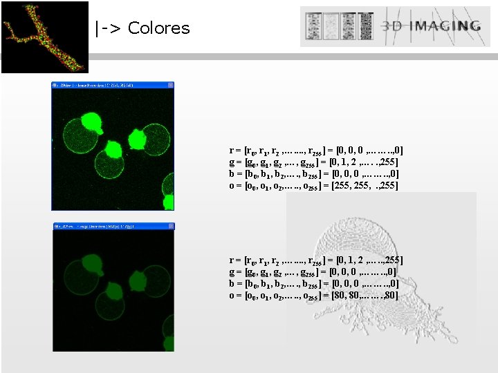
|-> Colores I(290, 267) = 220 r g 0 : : : 220 : : 255 b 0 : : : 220 : : 255 Cian (0, 255) Azul (0, 0, 255) Blanco (255, 255) Un canal tiene 8 bits y se pueden codificar 256 colores o intensidades Una mesa de color está definida por 3 vectores r, g, b de 8 bits. red = [r 0, r 1, …. . . , r 255] green = [g 0, g 1, ……. . . , g 255] blue = [b 0, b 1, ……. . . , b 255] Magenta (255, 0, 255) Verde (0, 255, 0) Negro (0, 0, 0) Rojo (255, 0, 0) Amarillo (255, 0)

|-> Colores r g 0 0 0 : : 0 0 1 2 : : 200 : : 255 b 0 0 0 : : 0

|-> Colores r g 0 1 2 : : 220 : : 255 0 0 0 : : 0 b 0 0 0 : : 0

|-> Colores

|-> Colores

|-> Colores

|-> Colores
 The standard error of the mean")
|-> Localization Standard error of the mean (SE) The standard error of the mean of a sample from a population is the standard deviation of the sampling distribution of the mean, and may be estimated by the formula: Where is an estimate of the standard deviation σ of the population, an n is the size (number of items) of the sample.

|-> ICA or ICQ ICA / ICQ Intensity Correlation Analysis /Quotient
![|-> ICQ Є [± 0. 5] Intensity Correlation Quotient One-Sample and Matched-Pairs tests •](http://slidetodoc.com/presentation_image_h2/93fad59d7b78ba8e5b5b9d0cc8775a53/image-40.jpg "|-> ICQ Є [± 0. 5] Intensity Correlation Quotient One-Sample and Matched-Pairs tests •")
|-> ICQ Є [± 0. 5] Intensity Correlation Quotient One-Sample and Matched-Pairs tests • Sign Test • Mc. Nemar's Test • Wilcoxon Matched-Pairs Signed-Ranks Test • Student-t test for one sample Sign Test p ≤ 0. 5 Σ ( N!/( i ! (N-i) ! )) i = 1, k (k = min(n+, n-))
")
|-> ICQ Sign Test p ≤ 0. 5 Σ ( N!/( i ! (N-i) ! )) i = 1, k (k = min(n+, n-)) Characteristics: Crudest and most insensitive test. It is also the most convincing and easiest to apply. The level of significance can almost be estimated without the help of a calculator or table. . . Approximation: For N > 30, the Student t-test can be used. However, the Wilcoxon Matched-Pairs Signed-Ranks test is a better alternative. Remarks: The Sign-test answers the question: How often? , whereas other tests answer the question How much? . It must be kept in mind that these two questions might have different answers. When the problem concerns the sizes of the differences, the Wilcoxon Matched-Pairs Signed. Ranks Test should be preferred. Finally, the Sign-test is an almost ideal quick-and-dirty test that can be used to browse datasets or to check the results of other tests (e. g. , as in: "All six subjects show an increase, so why does your test insist that p > 0. 05? "). http: //www. fon. hum. uva. nl/Service/Statistics/Sign_Test. html
- Slides: 41