HighPerformance Grid Computing and Research Networking HighPerformance Sequential

![Loop Constants n Identifying loop constants: for (k=0; k<N; k++) { c[i][j] += a[i][k] Loop Constants n Identifying loop constants: for (k=0; k<N; k++) { c[i][j] += a[i][k]](https://slidetodoc.com/presentation_image_h2/21fd8a8badec7f9598af66acca86db41/image-4.jpg)
![Address Computation n Example: a Mx. N row-major array j @(a[0][0]) X i i*N Address Computation n Example: a Mx. N row-major array j @(a[0][0]) X i i*N](https://slidetodoc.com/presentation_image_h2/21fd8a8badec7f9598af66acca86db41/image-10.jpg)
![Array Accesses are Expensive n Given that the formula is @(a[i][j]) = @(a[0][0]) + Array Accesses are Expensive n Given that the formula is @(a[i][j]) = @(a[0][0]) +](https://slidetodoc.com/presentation_image_h2/21fd8a8badec7f9598af66acca86db41/image-11.jpg)
![Loop Unrolling n Loop unrolling: for (i=0; i<100; i++) // 100 comparisons a[i] = Loop Unrolling n Loop unrolling: for (i=0; i<100; i++) // 100 comparisons a[i] =](https://slidetodoc.com/presentation_image_h2/21fd8a8badec7f9598af66acca86db41/image-13.jpg)
![Example n Source code: for(i=0; i<n; i++) sum += a[i] n Loop body in Example n Source code: for(i=0; i<n; i++) sum += a[i] n Loop body in](https://slidetodoc.com/presentation_image_h2/21fd8a8badec7f9598af66acca86db41/image-29.jpg)
![Other Techniques n Use more local variables while( … ) { *res++ = filter[0]*signal[0] Other Techniques n Use more local variables while( … ) { *res++ = filter[0]*signal[0]](https://slidetodoc.com/presentation_image_h2/21fd8a8badec7f9598af66acca86db41/image-37.jpg)
![Example #1: 2 -D Array Initialization int a[200]; for (i=0; i<200; i++) { for Example #1: 2 -D Array Initialization int a[200]; for (i=0; i<200; i++) { for](https://slidetodoc.com/presentation_image_h2/21fd8a8badec7f9598af66acca86db41/image-47.jpg)
![Row-Major n C uses Row-Major First option n int a[200]; for (i=0; i<200; i++) Row-Major n C uses Row-Major First option n int a[200]; for (i=0; i<200; i++)](https://slidetodoc.com/presentation_image_h2/21fd8a8badec7f9598af66acca86db41/image-48.jpg)
![Array Initialization in C First option n int a[200]; for (i=0; i<200; i++) for Array Initialization in C First option n int a[200]; for (i=0; i<200; i++) for](https://slidetodoc.com/presentation_image_h2/21fd8a8badec7f9598af66acca86db41/image-50.jpg)
![Performance Measurements n Option #1 int a[X][X]; for (i=0; i<200; i++) for (j=0; j<200; Performance Measurements n Option #1 int a[X][X]; for (i=0; i<200; i++) for (j=0; j<200;](https://slidetodoc.com/presentation_image_h2/21fd8a8badec7f9598af66acca86db41/image-51.jpg)
![Matrix Multiplication n A = [aij]i, j=1, . . . , N B = Matrix Multiplication n A = [aij]i, j=1, . . . , N B =](https://slidetodoc.com/presentation_image_h2/21fd8a8badec7f9598af66acca86db41/image-53.jpg)
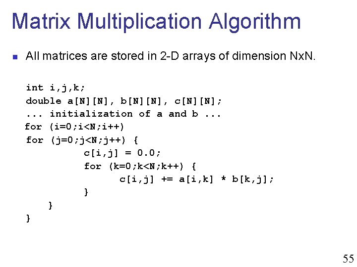
![First Performance Improvement for (i=0; i<N; i++) for (j=0; j<N; j++) { c[i][j] = First Performance Improvement for (i=0; i<N; i++) for (j=0; j<N; j++) { c[i][j] =](https://slidetodoc.com/presentation_image_h2/21fd8a8badec7f9598af66acca86db41/image-56.jpg)
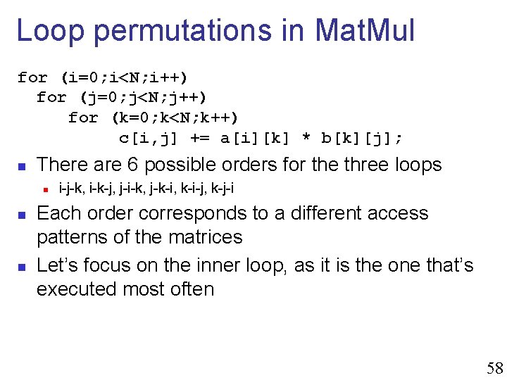
![Best Loop Ordering? c[i][j] i-j-k: Constant i-k-j: Sequential j-i-k: Constant j-k-i: Strided k-i-j: Sequential Best Loop Ordering? c[i][j] i-j-k: Constant i-k-j: Sequential j-i-k: Constant j-k-i: Strided k-i-j: Sequential](https://slidetodoc.com/presentation_image_h2/21fd8a8badec7f9598af66acca86db41/image-60.jpg)
- Slides: 89

High-Performance Grid Computing and Research Networking High-Performance Sequential Programming Presented by Juan Carlos Martinez Instructor: S. Masoud Sadjadi http: //www. cs. fiu. edu/~sadjadi/Teaching/ sadjadi At cs Dot fiu Dot edu 1

Acknowledgements n The content of many of the slides in this lecture notes have been adopted from the online resources prepared previously by the people listed below. Many thanks! n Henri Casanova n n n Principles of High Performance Computing http: //navet. ics. hawaii. edu/~casanova henric@hawaii. edu 2

Sequential Programs n n In this class we’re mostly focusing on concurrent programs But it’s useful to recall some simple notions of high performance for sequential programs n n n Because some fundamental techniques are meaningful for concurrent programs Because in your projects you’ll have to get code to go fast, and a concurrent program is just simultaneous sequential programs We’ll look at n n Standard code optimization techniques Optimizations dealing with memory issues 3
![Loop Constants n Identifying loop constants for k0 kN k cij aik Loop Constants n Identifying loop constants: for (k=0; k<N; k++) { c[i][j] += a[i][k]](https://slidetodoc.com/presentation_image_h2/21fd8a8badec7f9598af66acca86db41/image-4.jpg)
Loop Constants n Identifying loop constants: for (k=0; k<N; k++) { c[i][j] += a[i][k] * b[k][j]; } sum = 0; for (k=0; k<N; k++) { sum += a[i][k] * b[k][j]; } c[i][j] = sum; 4

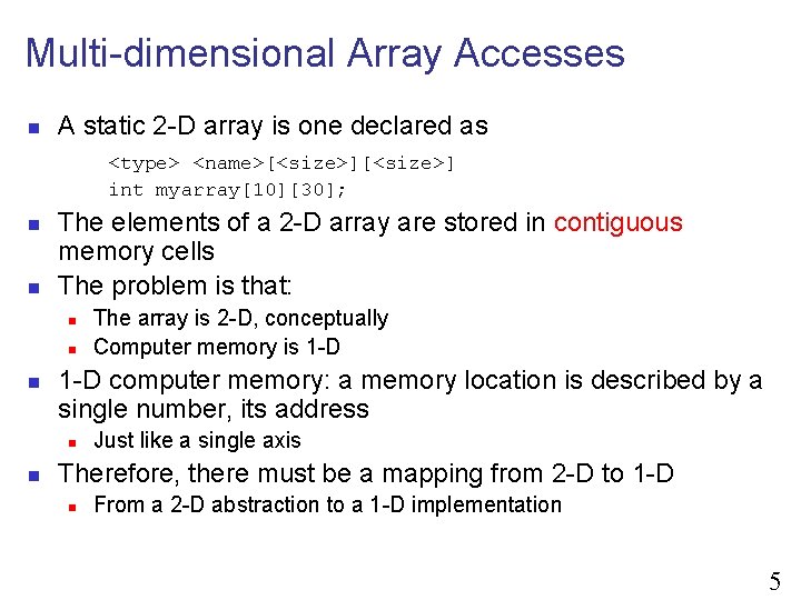
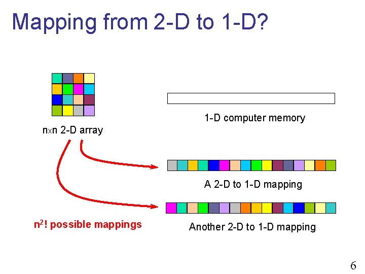
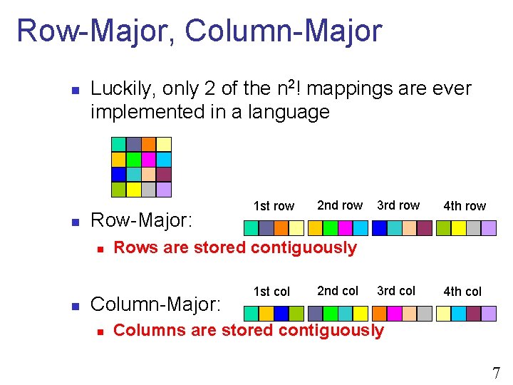
Multi-dimensional Array Accesses n A static 2 -D array is one declared as <type> <name>[<size>] int myarray[10][30]; n n The elements of a 2 -D array are stored in contiguous memory cells The problem is that: n n n 1 -D computer memory: a memory location is described by a single number, its address n n The array is 2 -D, conceptually Computer memory is 1 -D Just like a single axis Therefore, there must be a mapping from 2 -D to 1 -D n From a 2 -D abstraction to a 1 -D implementation 5

Mapping from 2 -D to 1 -D? 1 -D computer memory nxn 2 -D array A 2 -D to 1 -D mapping n 2! possible mappings Another 2 -D to 1 -D mapping 6

Row-Major, Column-Major n n Luckily, only 2 of the n 2! mappings are ever implemented in a language Row-Major: n n 2 nd row 3 rd row 4 th row 3 rd col 4 th col Rows are stored contiguously Column-Major: n 1 st row 1 st col 2 nd col Columns are stored contiguously 7

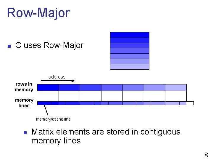
Row-Major n C uses Row-Major address rows in memory lines memory/cache line n Matrix elements are stored in contiguous memory lines 8

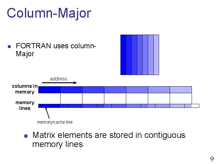
Column-Major n FORTRAN uses column. Major address columns in memory lines memory/cache line n Matrix elements are stored in contiguous memory lines 9
![Address Computation n Example a Mx N rowmajor array j a00 X i iN Address Computation n Example: a Mx. N row-major array j @(a[0][0]) X i i*N](https://slidetodoc.com/presentation_image_h2/21fd8a8badec7f9598af66acca86db41/image-10.jpg)
Address Computation n Example: a Mx. N row-major array j @(a[0][0]) X i i*N j M X N n Address Computation: @(a[i][j]) = @(a[0][0]) + i*N + j n n Example: n n Detail: there should be a sizeof() factor as well N = 6, M = 2 @(a[2][3]) = @(a[0][0]) + 2*6 + 3 = @(a[0][0]) + 15 For column-major (like in FORTRAN), the formula is reversed: n n @(a[i][j]) = @(a[0][0]) + j*M + i, or @(a[i][j]) = @(a[1][1]) + (j-1)*M + i-1 10
![Array Accesses are Expensive n Given that the formula is aij a00 Array Accesses are Expensive n Given that the formula is @(a[i][j]) = @(a[0][0]) +](https://slidetodoc.com/presentation_image_h2/21fd8a8badec7f9598af66acca86db41/image-11.jpg)
Array Accesses are Expensive n Given that the formula is @(a[i][j]) = @(a[0][0]) + i*N + j n Each array access entailed 2 additions and 1 multiplication n n This is even higher for higher dimension arrays Therefore, when the compiler compiles the instruction sum += a[i][k] * b[k][j]; n n 4 integer additions and 2 integer multiplications are generated just to compute addresses! And then 1 fp multiplication and 1 fp addition If the bottleneck is memory, then we don’t care But if the processor is not starved for data (which we will see is possible for this application), then the overhead of computing addresses is large 11

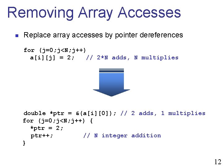
Removing Array Accesses n Replace array accesses by pointer dereferences for (j=0; j<N; j++) a[i][j] = 2; // 2*N adds, N multiplies double *ptr = &(a[i][0]); // 2 adds, 1 multiplies for (j=0; j<N; j++) { *ptr = 2; ptr++; // N integer addition } 12
![Loop Unrolling n Loop unrolling for i0 i100 i 100 comparisons ai Loop Unrolling n Loop unrolling: for (i=0; i<100; i++) // 100 comparisons a[i] =](https://slidetodoc.com/presentation_image_h2/21fd8a8badec7f9598af66acca86db41/image-13.jpg)
Loop Unrolling n Loop unrolling: for (i=0; i<100; i++) // 100 comparisons a[i] = i; i=0; do { a[i] = i; i++; } while (i<100) // 25 comparisons 13

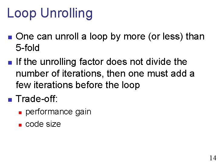
Loop Unrolling n n n One can unroll a loop by more (or less) than 5 -fold If the unrolling factor does not divide the number of iterations, then one must add a few iterations before the loop Trade-off: n n performance gain code size 14

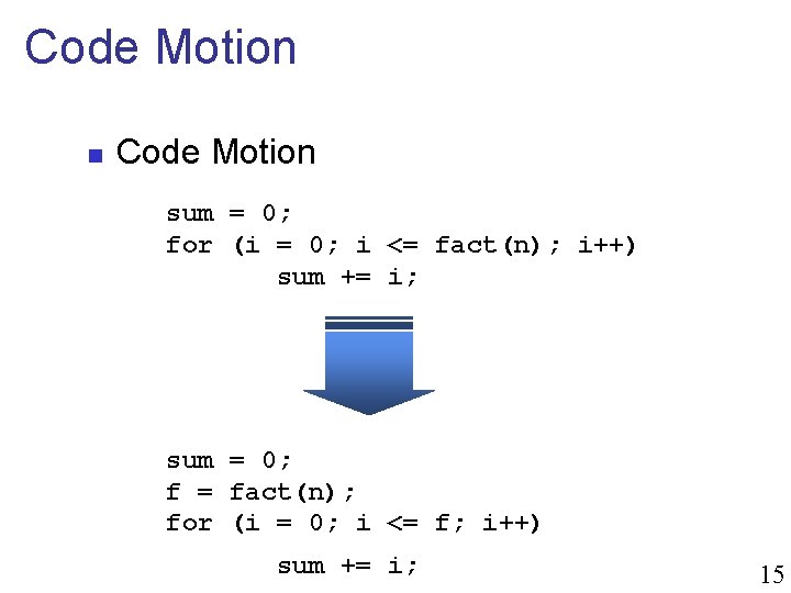
Code Motion n Code Motion sum = 0; for (i = 0; i <= fact(n); i++) sum += i; sum = 0; f = fact(n); for (i = 0; i <= f; i++) sum += i; 15

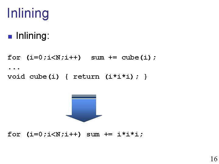
Inlining n Inlining: for (i=0; i<N; i++) sum += cube(i); . . . void cube(i) { return (i*i*i); } for (i=0; i<N; i++) sum += i*i*i; 16

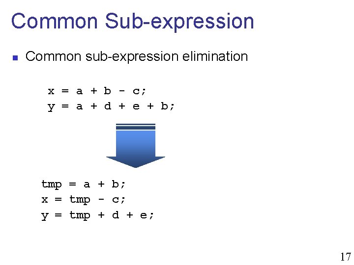
Common Sub-expression n Common sub-expression elimination x = a + b - c; y = a + d + e + b; tmp = a + b; x = tmp - c; y = tmp + d + e; 17

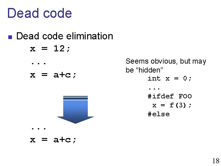
Dead code n Dead code elimination x = 12; . . . x = a+c; Seems obvious, but may be “hidden” int x = 0; . . . #ifdef FOO x = f(3); #else . . . x = a+c; 18

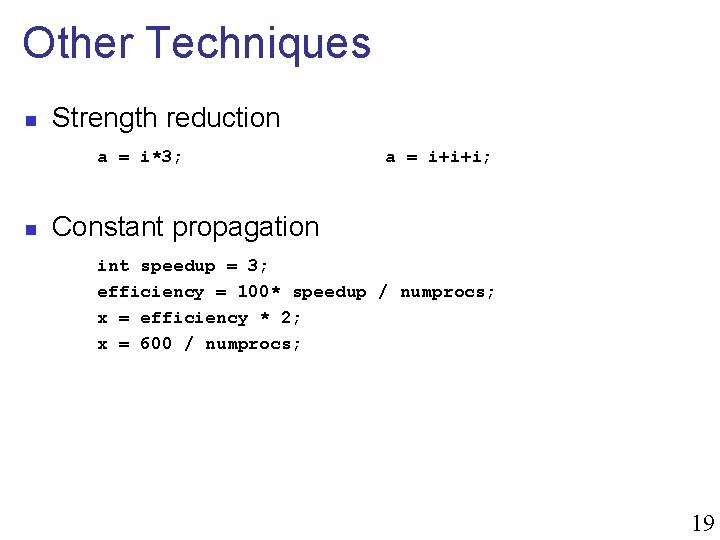
Other Techniques n Strength reduction a = i*3; n a = i+i+i; Constant propagation int speedup = 3; efficiency = 100* speedup / numprocs; x = efficiency * 2; x = 600 / numprocs; 19

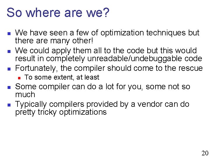
So where are we? n n n We have seen a few of optimization techniques but there are many other! We could apply them all to the code but this would result in completely unreadable/undebuggable code Fortunately, the compiler should come to the rescue n n n To some extent, at least Some compiler can do a lot for you, some not so much Typically compilers provided by a vendor can do pretty tricky optimizations 20

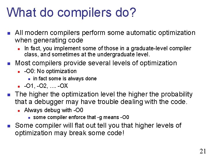
What do compilers do? n All modern compilers perform some automatic optimization when generating code n n In fact, you implement some of those in a graduate-level compiler class, and sometimes at the undergraduate level. Most compilers provide several levels of optimization n -O 0: No optimization n -O 1, -O 2, . . -OX The higher the optimization level the higher the probability that a debugger may have trouble dealing with the code. n Always debug with -O 0 n n in fact some is always done some compiler enforce that -g means -O 0 Some compiler will flat out tell you that higher levels of optimization may break some code! 21

Compiler optimizations n In this class we use gcc, which is free and pretty good n -Os: Optimize for size n n Do a “man gcc” and look at the many optimization options n n n Some optimizations increase code size tremendously one can pick and choose, or just use standard sets via O 1, O 2, etc. The most fancy compilers are typically the ones done by vendors n n You can’t sell a good machine if it has a bad compiler Compiler technology used to be really poor also, languages used to be designed without thinking of compilers (FORTRAN, Ada) no longer true: every language designer has in-depth understanding of compiler technology today 22

What can compilers do? n Most of the techniques we’ve seen!! n n Inlining Assignment of variables to registers n n n n Dead code elimination Algebraic simplification Moving invariant code out of loops Constant propagation Control flow simplification Instruction scheduling, reordering Strength reduction n n It’s a difficult problem e. g. , add to pointers, rather than doing array index computation Loop unrolling and software pipelining Dead store elimination and many other. . . 23

What can compilers do? n Most of the techniques we’ve seen!! n n Inlining Assignment of variables to registers n n n n Dead code elimination Algebraic simplification Moving invariant code out of loops Constant propagation Control flow simplification Instruction scheduling, reordering Strength reduction n n It’s a difficult problem e. g. , add to pointers, rather than doing array index computation Loop unrolling and software pipelining Dead store elimination and many other. . . 24

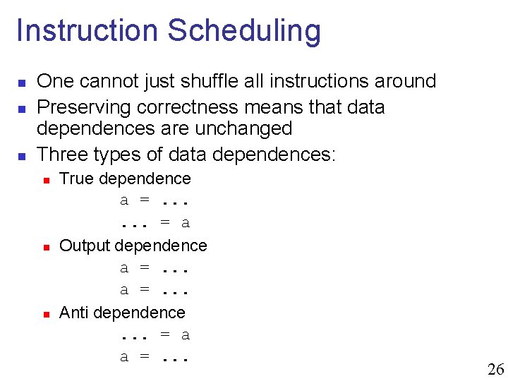
Instruction scheduling n n Modern computers have multiple functional units that could be used in parallel Or at least ones that are pipelined n n n if fed operands at each cycle they can produce a result at each cycle although a computation may require 20 cycles Instruction scheduling: n Reorder the instructions of a program n n n e. g. , at the assembly code level Preserve correctness Make it possible to use functional units optimally 25

Instruction Scheduling n n n One cannot just shuffle all instructions around Preserving correctness means that data dependences are unchanged Three types of data dependences: n n n True dependence a =. . . = a Output dependence a =. . . Anti dependence. . . = a a =. . . 26

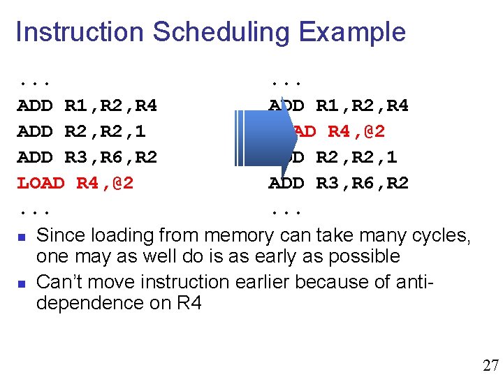
Instruction Scheduling Example. . . ADD R 1, R 2, R 4 ADD R 2, 1 LOAD R 4, @2 ADD R 3, R 6, R 2. . . n Since loading from memory can take many cycles, one may as well do is as early as possible n Can’t move instruction earlier because of antidependence on R 4 27

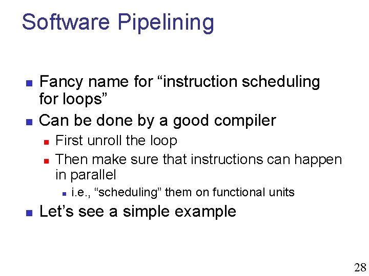
Software Pipelining n n Fancy name for “instruction scheduling for loops” Can be done by a good compiler n n First unroll the loop Then make sure that instructions can happen in parallel n n i. e. , “scheduling” them on functional units Let’s see a simple example 28
![Example n Source code fori0 in i sum ai n Loop body in Example n Source code: for(i=0; i<n; i++) sum += a[i] n Loop body in](https://slidetodoc.com/presentation_image_h2/21fd8a8badec7f9598af66acca86db41/image-29.jpg)
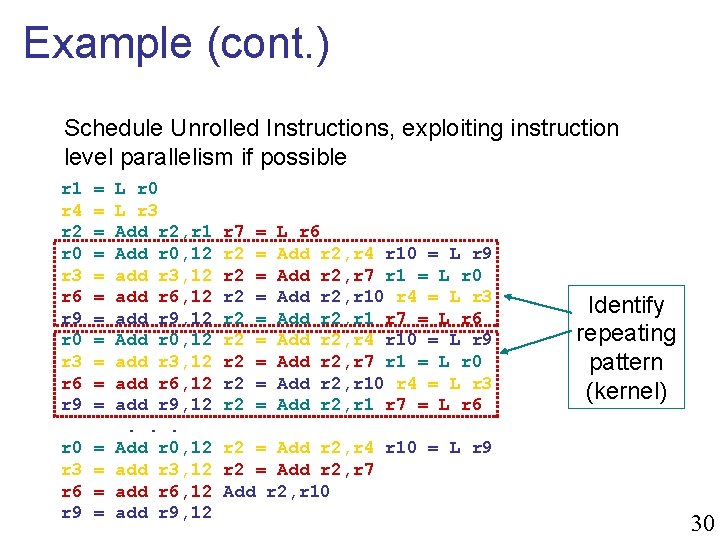
Example n Source code: for(i=0; i<n; i++) sum += a[i] n Loop body in assembly: r 1 = L r 0 --- ; stall r 2 = Add r 2, r 1 r 0 = add r 0, 4 n Unroll loop & allocate registers n May be very difficult r 1 = L r 0 --- ; stall r 2 = Add r 2, r 1 r 0 = Add r 0, 12 r 4 = L r 3 --- ; stall r 2 = Add r 2, r 4 r 3 = add r 3, 12 r 7 = L r 6 --- ; stall r 2 = Add r 2, r 7 r 6 = add r 6, 12 r 10 = L r 9 --- ; stall r 2 = Add r 2, r 10 r 9 = add r 9, 12 29

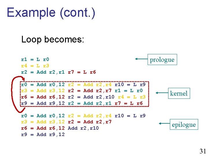
Example (cont. ) Schedule Unrolled Instructions, exploiting instruction level parallelism if possible r 1 r 4 r 2 r 0 r 3 r 6 r 9 = = = r 0 r 3 r 6 r 9 = = L r 0 L r 3 Add r 2, r 1 Add r 0, 12 add r 3, 12 add r 6, 12 add r 9, 12. . . Add r 0, 12 add r 3, 12 add r 6, 12 add r 9, 12 r 7 r 2 r 2 = = = = = L r 6 Add r 2, r 4 r 10 = L r 9 Add r 2, r 7 r 1 = L r 0 Add r 2, r 10 r 4 = L r 3 Add r 2, r 1 r 7 = L r 6 Identify repeating pattern (kernel) r 2 = Add r 2, r 4 r 10 = L r 9 r 2 = Add r 2, r 7 Add r 2, r 10 30

Example (cont. ) Loop becomes: prologue r 1 = L r 0 r 4 = L r 3 r 2 = Add r 2, r 1 r 7 = L r 6 r 0 r 3 r 6 r 9 = = Add Add r 0, 12 r 3, 12 r 6, 12 r 9, 12 r 2 r 2 = = Add Add r 2, r 4 r 10 = L r 9 r 2, r 7 r 1 = L r 0 r 2, r 10 r 4 = L r 3 r 2, r 1 r 7 = L r 6 r 0 r 3 r 6 r 9 = = Add Add r 0, 12 r 2 = Add r 2, r 4 r 10 = L r 9 r 3, 12 r 2 = Add r 2, r 7 r 6, 12 Add r 2, r 10 r 9, 12 kernel epilogue 31

Software Pipelining n The “kernel” may require many registers and it’s nice to know how to use as few as possible n n Dependency constraints must be respected n n otherwise, one may have to go to cache more, which may negate the benefits of software pipelining May be very difficult to analyze for complex nested loops Software pipelining with registers is a very well-known NPhard program 32

Limits to Compiler Optimization n Behavior that may be obvious to the programmer can be obfuscated by languages and coding styles n e. g. , data ranges may be more limited than variable types suggest n n Most analysis is performed only within procedures n n whole-program analysis is too expensive in most cases Most analysis is based only on static information n n e. g. , using an “int” in C for what could be an enumerated type compiler has difficulty anticipating run-time inputs When in doubt, the compiler must be conservative n cannot perform optimization if it changes program behavior under any realizable circumstance n even if circumstances seem quite bizarre and unlikely 33

Good practice n n Writing code for high performance means working hand-in-hand with the compiler #1: Optimize things that we know the compiler cannot deal with n n n For instance the “blocking” optimization for matrix multiplication may need to be done by hand But some compiler may find the best i-j-k ordering!! #2: Write code so that the compiler can do its optimizations n Remove optimization blockers 34

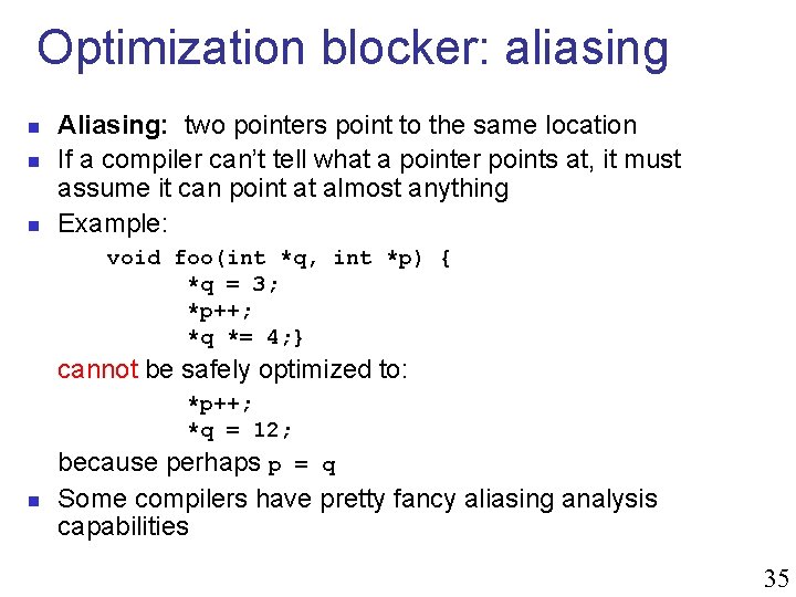
Optimization blocker: aliasing n n n Aliasing: two pointers point to the same location If a compiler can’t tell what a pointer points at, it must assume it can point at almost anything Example: void foo(int *q, int *p) { *q = 3; *p++; *q *= 4; } cannot be safely optimized to: *p++; *q = 12; n because perhaps p = q Some compilers have pretty fancy aliasing analysis capabilities 35

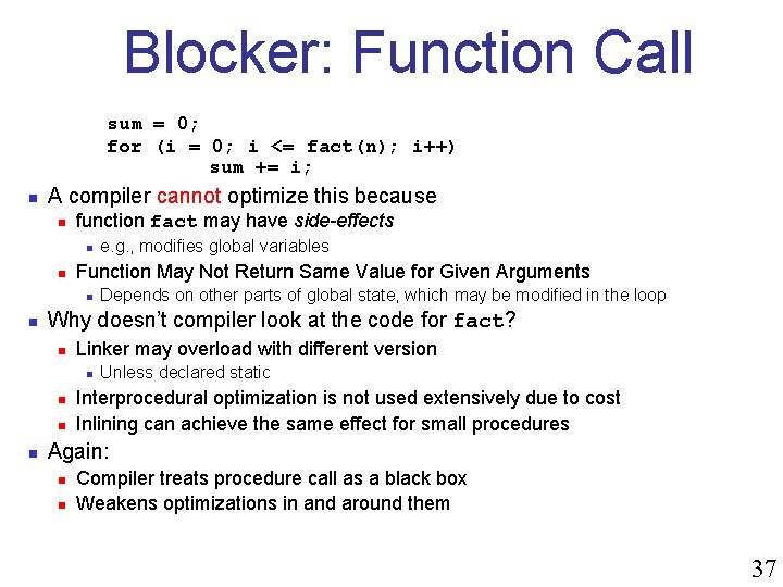
Blocker: Function Call sum = 0; for (i = 0; i <= fact(n); i++) sum += i; n A compiler cannot optimize this because n function fact may have side-effects n n Function May Not Return Same Value for Given Arguments n n Depends on other parts of global state, which may be modified in the loop Why doesn’t compiler look at the code for fact? n Linker may overload with different version n n e. g. , modifies global variables Unless declared static Interprocedural optimization is not used extensively due to cost Inlining can achieve the same effect for small procedures Again: n n Compiler treats procedure call as a black box Weakens optimizations in and around them 37
![Other Techniques n Use more local variables while res filter0signal0 Other Techniques n Use more local variables while( … ) { *res++ = filter[0]*signal[0]](https://slidetodoc.com/presentation_image_h2/21fd8a8badec7f9598af66acca86db41/image-37.jpg)
Other Techniques n Use more local variables while( … ) { *res++ = filter[0]*signal[0] + filter[1]*signal[1] + filter[2]*signal[2]; signal++; } Helps some compilers register float f 0 = filter[0]; register float f 1 = filter[1]; register float f 2 = filter[2]; while( … ) { *res++ = f 0*signal[0] + f 1*signal[1] + f 2*signal[2]; signal++; } 38

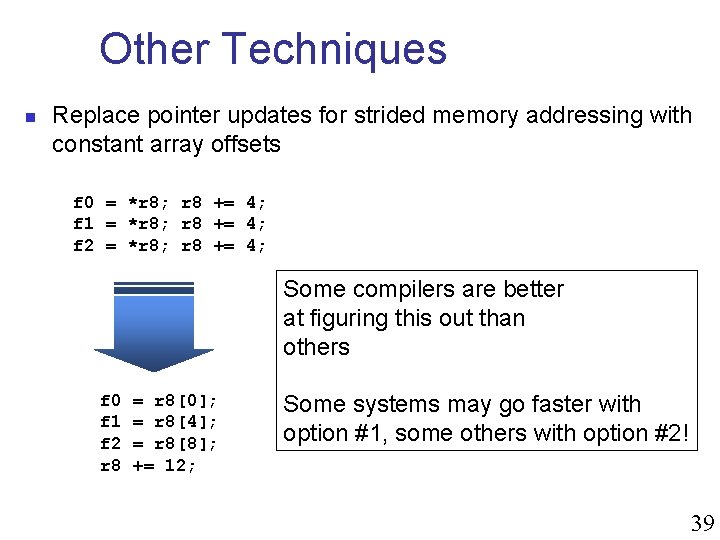
Other Techniques n Replace pointer updates for strided memory addressing with constant array offsets f 0 = *r 8; r 8 += 4; f 1 = *r 8; r 8 += 4; f 2 = *r 8; r 8 += 4; Some compilers are better at figuring this out than others f 0 f 1 f 2 r 8 = r 8[0]; = r 8[4]; = r 8[8]; += 12; Some systems may go faster with option #1, some others with option #2! 39

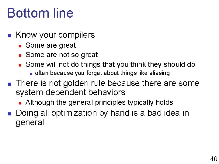
Bottom line n Know your compilers n n n Some are great Some are not so great Some will not do things that you think they should do n n There is not golden rule because there are some system-dependent behaviors n n often because you forget about things like aliasing Although the general principles typically holds Doing all optimization by hand is a bad idea in general 40

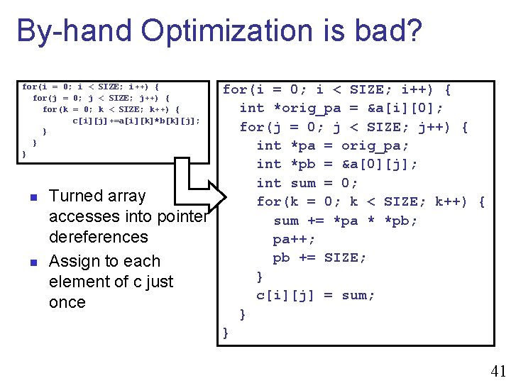
By-hand Optimization is bad? for(i = 0; i < SIZE; i++) { for(j = 0; j < SIZE; j++) { for(k = 0; k < SIZE; k++) { c[i][j]+=a[i][k]*b[k][j]; } } } n n Turned array accesses into pointer dereferences Assign to each element of c just once for(i = 0; i < SIZE; i++) { int *orig_pa = &a[i][0]; for(j = 0; j < SIZE; j++) { int *pa = orig_pa; int *pb = &a[0][j]; int sum = 0; for(k = 0; k < SIZE; k++) { sum += *pa * *pb; pa++; pb += SIZE; } c[i][j] = sum; } } 41

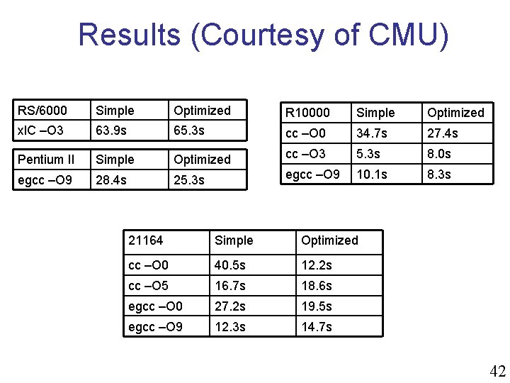
Results (Courtesy of CMU) RS/6000 Simple Optimized R 10000 Simple Optimized xl. C –O 3 63. 9 s 65. 3 s cc –O 0 34. 7 s 27. 4 s Pentium II Simple Optimized cc –O 3 5. 3 s 8. 0 s egcc –O 9 28. 4 s 25. 3 s egcc –O 9 10. 1 s 8. 3 s 21164 Simple Optimized cc –O 0 40. 5 s 12. 2 s cc –O 5 16. 7 s 18. 6 s egcc –O 0 27. 2 s 19. 5 s egcc –O 9 12. 3 s 14. 7 s 42

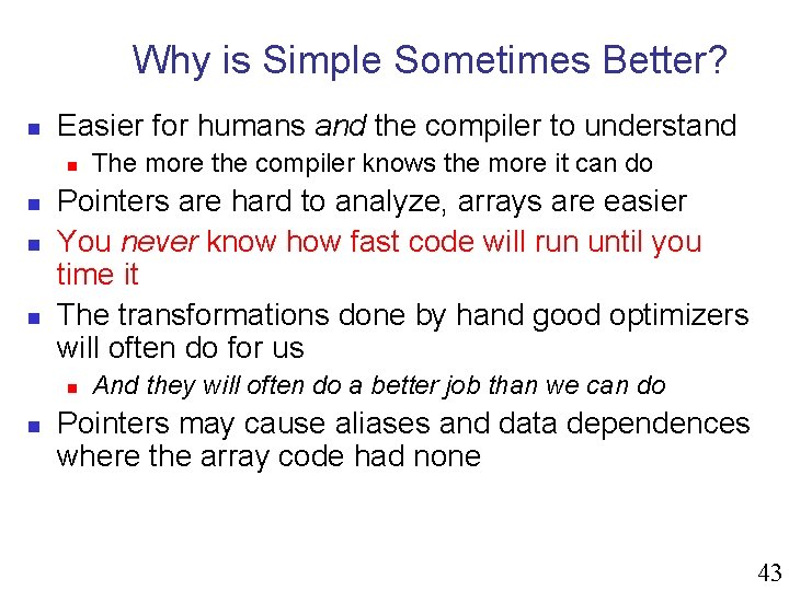
Why is Simple Sometimes Better? n Easier for humans and the compiler to understand n n Pointers are hard to analyze, arrays are easier You never know how fast code will run until you time it The transformations done by hand good optimizers will often do for us n n The more the compiler knows the more it can do And they will often do a better job than we can do Pointers may cause aliases and data dependences where the array code had none 43

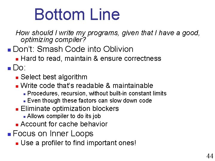
Bottom Line How should I write my programs, given that I have a good, optimizing compiler? n Don’t: Smash Code into Oblivion n n Hard to read, maintain & ensure correctness Do: n n Select best algorithm Write code that’s readable & maintainable Procedures, recursion, without built-in constant limits n Even though these factors can slow down code n n Eliminate optimization blockers n n n Allows compiler to do its job Account for cache behavior Focus on Inner Loops n Use a profiler to find important ones! 44

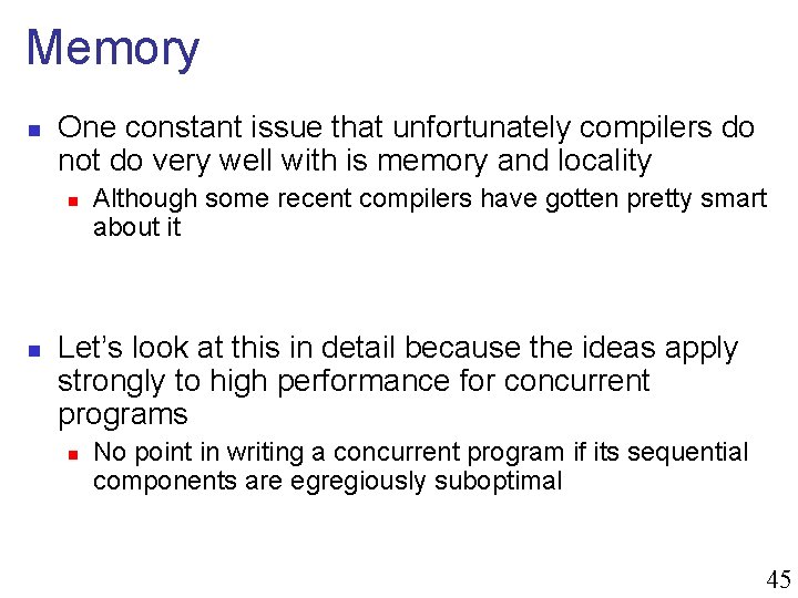
Memory n One constant issue that unfortunately compilers do not do very well with is memory and locality n n Although some recent compilers have gotten pretty smart about it Let’s look at this in detail because the ideas apply strongly to high performance for concurrent programs n No point in writing a concurrent program if its sequential components are egregiously suboptimal 45

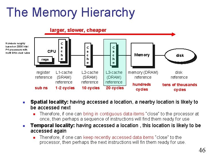
The Memory Hierarchy larger, slower, cheaper Numbers roughly based on 2005 Intel P 4 processors with multi GHz clock rates CPU regs C a c h e register L 1 -cache reference (SRAM) reference sub ns 1 -2 cycles n L 2 -cache (SRAM) reference 10 cycles C a c h e Memory L 3 -cache memory (DRAM) reference hundreds 20 cycles disk reference tens of thousands cycles Spatial locality: having accessed a location, a nearby location is likely to be accessed next n n C a c h e Therefore, if one can bring in contiguous data items “close” to the processor at once, then perhaps a sequence of instructions will find them ready for use Temporal locality: having accessed a location , this location is likely to be accessed again n Therefore, if one can keep recently accessed data items “close” to the processor, then perhaps the next instructions will fin them ready for use. 46

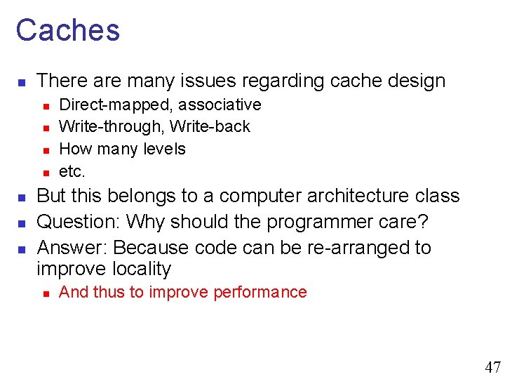
Caches n There are many issues regarding cache design n n n Direct-mapped, associative Write-through, Write-back How many levels etc. But this belongs to a computer architecture class Question: Why should the programmer care? Answer: Because code can be re-arranged to improve locality n And thus to improve performance 47
![Example 1 2 D Array Initialization int a200 for i0 i200 i for Example #1: 2 -D Array Initialization int a[200]; for (i=0; i<200; i++) { for](https://slidetodoc.com/presentation_image_h2/21fd8a8badec7f9598af66acca86db41/image-47.jpg)
Example #1: 2 -D Array Initialization int a[200]; for (i=0; i<200; i++) { for (j=0; j<200; j++) { a[i][j] = 2; } } n Which alternative is best? n n n int a[200]; for (j=0; j<200; j++) { for (i=0; i<200; i++) { a[i][j] = 2; } } i, j? j, i? To answer this, one must understand the memory layout of a 2 -D array 48
![RowMajor n C uses RowMajor First option n int a200 for i0 i200 i Row-Major n C uses Row-Major First option n int a[200]; for (i=0; i<200; i++)](https://slidetodoc.com/presentation_image_h2/21fd8a8badec7f9598af66acca86db41/image-48.jpg)
Row-Major n C uses Row-Major First option n int a[200]; for (i=0; i<200; i++) for (j=0; j<200; j++) a[i][j]=2; Second option n int a[200]; for (i=0; i<200; i++) for (j=0; j<200; j++) a[i][j]=2; 49

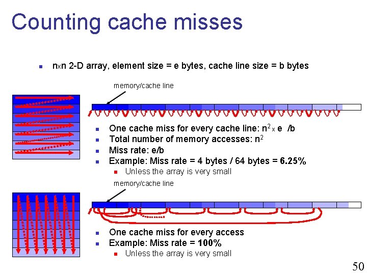
Counting cache misses n nxn 2 -D array, element size = e bytes, cache line size = b bytes memory/cache line n n One cache miss for every cache line: n 2 x e /b Total number of memory accesses: n 2 Miss rate: e/b Example: Miss rate = 4 bytes / 64 bytes = 6. 25% n Unless the array is very small memory/cache line n n One cache miss for every access Example: Miss rate = 100% n Unless the array is very small 50
![Array Initialization in C First option n int a200 for i0 i200 i for Array Initialization in C First option n int a[200]; for (i=0; i<200; i++) for](https://slidetodoc.com/presentation_image_h2/21fd8a8badec7f9598af66acca86db41/image-50.jpg)
Array Initialization in C First option n int a[200]; for (i=0; i<200; i++) for (j=0; j<200; j++) a[i][j]=2; Good Locality Second option n int a[200]; for (i=0; i<200; i++) for (j=0; j<200; j++) a[i][j]=2; 51
![Performance Measurements n Option 1 int aXX for i0 i200 i for j0 j200 Performance Measurements n Option #1 int a[X][X]; for (i=0; i<200; i++) for (j=0; j<200;](https://slidetodoc.com/presentation_image_h2/21fd8a8badec7f9598af66acca86db41/image-51.jpg)
Performance Measurements n Option #1 int a[X][X]; for (i=0; i<200; i++) for (j=0; j<200; j++) a[i][j]=2; n Option #2 int a[X][X]; for (j=0; j<200; j++) for (i=0; i<200; i++) a[i][j]=2; Experiments on my laptop n Note that other languages use column major n e. g. , FORTRAN 52

Matrix Multiplication n The previous example was very simple But things can get more complicated very quickly Let’s look at a simple program to multiply two square matrices n A fundamental operation in linear algebra n n Linear system resolution Computing the transitive closure of a graph etc. Probably the most well-studied problem in HPC n n clever algorithms clever implementations 53
![Matrix Multiplication n A aiji j1 N B Matrix Multiplication n A = [aij]i, j=1, . . . , N B =](https://slidetodoc.com/presentation_image_h2/21fd8a8badec7f9598af66acca86db41/image-53.jpg)
Matrix Multiplication n A = [aij]i, j=1, . . . , N B = [bij]i, j=1, . . . , N C = A x B = [cij]i, j=1, . . . , N b 1 i x ai 1 b 2 i x ai 2 . . Like most linear algebra operations, this formula can be translated into a very simple computer program that just “follows” the math . i j cij 54

Matrix Multiplication Algorithm n All matrices are stored in 2 -D arrays of dimension Nx. N. int i, j, k; double a[N][N], b[N][N], c[N][N]; . . . initialization of a and b. . . for (i=0; i<N; i++) for (j=0; j<N; j++) { c[i, j] = 0. 0; for (k=0; k<N; k++) { c[i, j] += a[i, k] * b[k, j]; } } } 55

How good is this algorithm? n This algorithm is good because: n n n It takes only a few lines It is a direct mapping to the formula for cij Anybody should be able to understand what it does by just looking at it It almost certainly has no bug because it is so simple This algorithm is bad because: n It has terrible performance because it ignores the fact that the underlying computer has a memory hierarchy 56
![First Performance Improvement for i0 iN i for j0 jN j cij First Performance Improvement for (i=0; i<N; i++) for (j=0; j<N; j++) { c[i][j] =](https://slidetodoc.com/presentation_image_h2/21fd8a8badec7f9598af66acca86db41/image-56.jpg)
First Performance Improvement for (i=0; i<N; i++) for (j=0; j<N; j++) { c[i][j] = 0. 0; for (k=0; k<N; k++) { c[i][j] += a[i][k] * b[k][j]; } } } n n Note that it is assume the compiler will remove c[i][j] form the inner loop, unroll loops, etc. First idea: Switching loops around? n After all it worked for array initialization 57

Loop permutations in Mat. Mul for (i=0; i<N; i++) for (j=0; j<N; j++) for (k=0; k<N; k++) c[i, j] += a[i][k] * b[k][j]; n There are 6 possible orders for the three loops n n n i-j-k, i-k-j, j-i-k, j-k-i, k-i-j, k-j-i Each order corresponds to a different access patterns of the matrices Let’s focus on the inner loop, as it is the one that’s executed most often 58

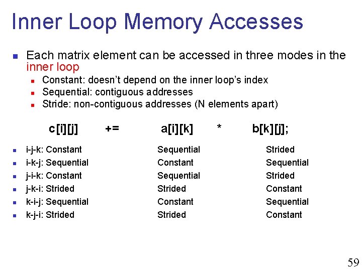
Inner Loop Memory Accesses n Each matrix element can be accessed in three modes in the inner loop n n n Constant: doesn’t depend on the inner loop’s index Sequential: contiguous addresses Stride: non-contiguous addresses (N elements apart) c[i][j] n n n i-j-k: Constant i-k-j: Sequential j-i-k: Constant j-k-i: Strided k-i-j: Sequential k-j-i: Strided += a[i][k] Sequential Constant Sequential Strided Constant Strided * b[k][j]; Strided Sequential Strided Constant Sequential Constant 59

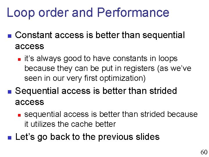
Loop order and Performance n Constant access is better than sequential access n n Sequential access is better than strided access n n it’s always good to have constants in loops because they can be put in registers (as we’ve seen in our very first optimization) sequential access is better than strided because it utilizes the cache better Let’s go back to the previous slides 60
![Best Loop Ordering cij ijk Constant ikj Sequential jik Constant jki Strided kij Sequential Best Loop Ordering? c[i][j] i-j-k: Constant i-k-j: Sequential j-i-k: Constant j-k-i: Strided k-i-j: Sequential](https://slidetodoc.com/presentation_image_h2/21fd8a8badec7f9598af66acca86db41/image-60.jpg)
Best Loop Ordering? c[i][j] i-j-k: Constant i-k-j: Sequential j-i-k: Constant j-k-i: Strided k-i-j: Sequential k-j-i: Strided += a[i][k] * Sequential Constant Sequential Strided Constant Strided b[k][j]; Strided Sequential Strided Constant Sequential Constant n k-i-j and i-k-j should have the best performance i-j-k and j-i-k should be worse j-k-i and k-j-i should be the worst n You will measure this in the first (warm-up) assignment n n 61

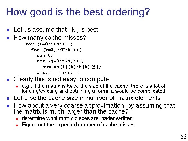
How good is the best ordering? n n Let us assume that i-k-j is best How many cache misses? for (i=0; i<N; i++) for (k=0; k<N; k++){ sum=0; for (j=0; j<N; j++) sum+=a[i][k]*b[k][j]; c[i, j] = sum; } n Clearly this is not easy to compute n n n e. g. , if the matrix is twice the size of the cache, there is a lot of loading/evicting and obtaining a formula would be complicated Let L be the cache size in number of matrix elements How about a very coarse approximation, by assuming that the matrix is much larger than the cache? n n determine what matrix pieces are loaded/written Figure out the expected number of cache misses 62

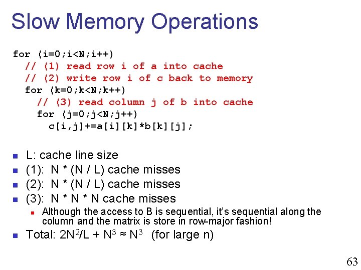
Slow Memory Operations for (i=0; i<N; i++) // (1) read row i of a into cache // (2) write row i of c back to memory for (k=0; k<N; k++) // (3) read column j of b into cache for (j=0; j<N; j++) c[i, j]+=a[i][k]*b[k][j]; n n L: cache line size (1): N * (N / L) cache misses (2): N * (N / L) cache misses (3): N * N cache misses n n Although the access to B is sequential, it’s sequential along the column and the matrix is store in row-major fashion! Total: 2 N 2/L + N 3 ≈ N 3 (for large n) 63

Bad News n n n ≈ N 3 slow memory operations and 2 N 3 arithmetic operations Ratio ops / mem ≈ 2 This is bad news because we know that computer architectures are NOT balanced and memory operations are orders of magnitude slower than arithmetic operations Therefore, the memory is still the bottleneck for this implementation of matrix multiplication (the ratio should be much higher) BUT: we have only N 2 matrix elements, how come we perform N 3 slow memory accesses? n n Because we access matrix B very inefficiently, trying to load entire columns one after the other Lesson: counting the number of operations and comparing it with the size of the data is not sufficient to ascertain that an algorithm will not suffer from the memory bottleneck 64

Better cache reuse? n Since we really need only N 2 elements, perhaps there is a better way to reorganize the operations of the matrix multiplication for a higher number of cache hits n n n Possible because ‘+’ and ‘*’ are associative and commutative Researchers have spent a lot of time trying to find out the best ordering There are even theorems! n n n Let q = ratio of operations to slow memory accesses q must be as high as possible to remove the memory bottleneck [Hong&Kung 1981] Any reorganization of the algorithm is limited to q = O(√M), where M is the size of the cache (in number of elements) n n obtained with a lot of unrealistic assumptions about the cache still shows that q won’t scale with N, unlike what one may think when dividing 2 n 3 by n 2. 65

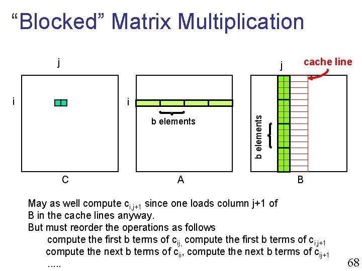
“Blocked” Matrix Multiplication n n One problem with our implementation is that we try to access entire columns of matrix B. What about accessing only a subset of a column, or of multiple columns, at a time? 66

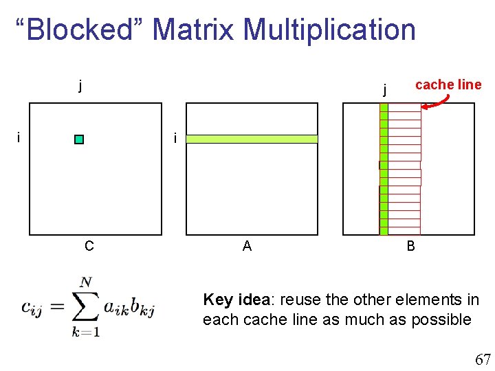
“Blocked” Matrix Multiplication j j i cache line i C A B Key idea: reuse the other elements in each cache line as much as possible 67

“Blocked” Matrix Multiplication j j i cache line b elements C A b elements i B May as well compute ci, j+1 since one loads column j+1 of B in the cache lines anyway. But must reorder the operations as follows compute the first b terms of cij, compute the first b terms of ci, j+1 compute the next b terms of cii, compute the next b terms of cij+1. . . 68

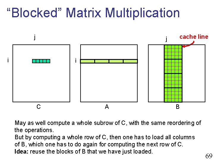
“Blocked” Matrix Multiplication j j i cache line i C A B May as well compute a whole subrow of C, with the same reordering of the operations. But by computing a whole row of C, then one has to load all columns of B, which one has to do again for computing the next row of C. Idea: reuse the blocks of B that we have just loaded. 69

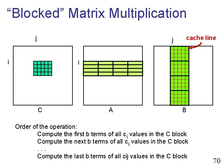
“Blocked” Matrix Multiplication j j i cache line i C A B Order of the operation: Compute the first b terms of all cij values in the C block Compute the next b terms of all cij values in the C block. . . Compute the last b terms of all cij values in the C block 70

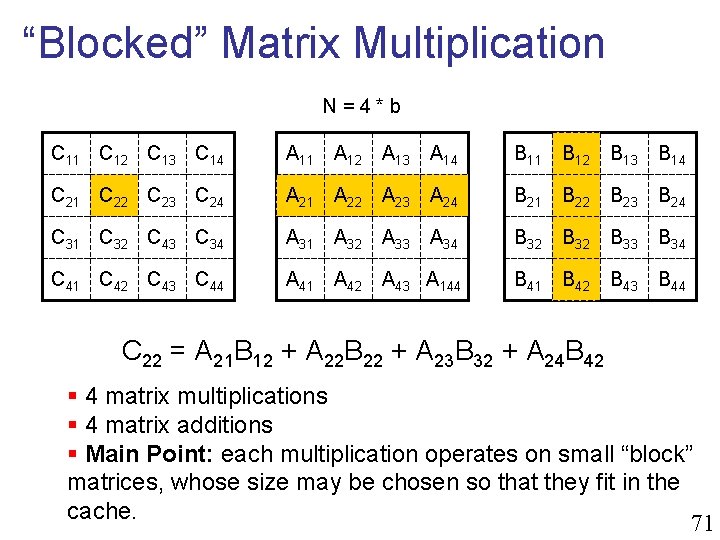
“Blocked” Matrix Multiplication N=4*b C 11 C 12 C 13 C 14 A 11 A 12 A 13 A 14 B 11 B 12 B 13 B 14 C 21 C 22 C 23 C 24 A 21 A 22 A 23 A 24 B 21 B 22 B 23 B 24 C 31 C 32 C 43 C 34 A 31 A 32 A 33 A 34 B 32 B 33 B 34 C 41 C 42 C 43 C 44 A 41 A 42 A 43 A 144 B 41 B 42 B 43 B 44 C 22 = A 21 B 12 + A 22 B 22 + A 23 B 32 + A 24 B 42 § 4 matrix multiplications § 4 matrix additions § Main Point: each multiplication operates on small “block” matrices, whose size may be chosen so that they fit in the cache. 71

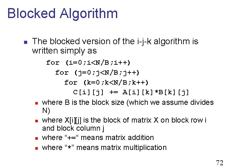
Blocked Algorithm n The blocked version of the i-j-k algorithm is written simply as n n for (i=0; i<N/B; i++) for (j=0; j<N/B; j++) for (k=0; k<N/B; k++) C[i][j] += A[i][k]*B[k][j] where B is the block size (which we assume divides N) where X[i][j] is the block of matrix X on block row i and block column j where “+=“ means matrix addition where “*” means matrix multiplication 72

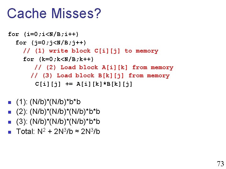
Cache Misses? for (i=0; i<N/B; i++) for (j=0; j<N/B; j++) // (1) write block C[i][j] to memory for (k=0; k<N/B; k++) // (2) Load block A[i][k] from memory // (3) Load block B[k][j] from memory C[i][j] += A[i][k]*B[k][j] n n (1): (N/b)*b*b (2): (N/b)*(N/b)*b*b (3): (N/b)*(N/b)*b*b Total: N 2 + 2 N 3/b ≈ 2 N 3/b 73

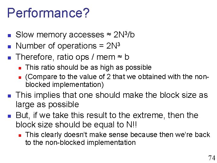
Performance? n n n Slow memory accesses ≈ 2 N 3/b Number of operations = 2 N 3 Therefore, ratio ops / mem ≈ b n n This ratio should be as high as possible (Compare to the value of 2 that we obtained with the nonblocked implementation) This implies that one should make the block size as large as possible But, if we take this result to the extreme, then the block size should be equal to N!! n This clearly doesn’t make sense because then we’re back to the non-blocked implementation 74

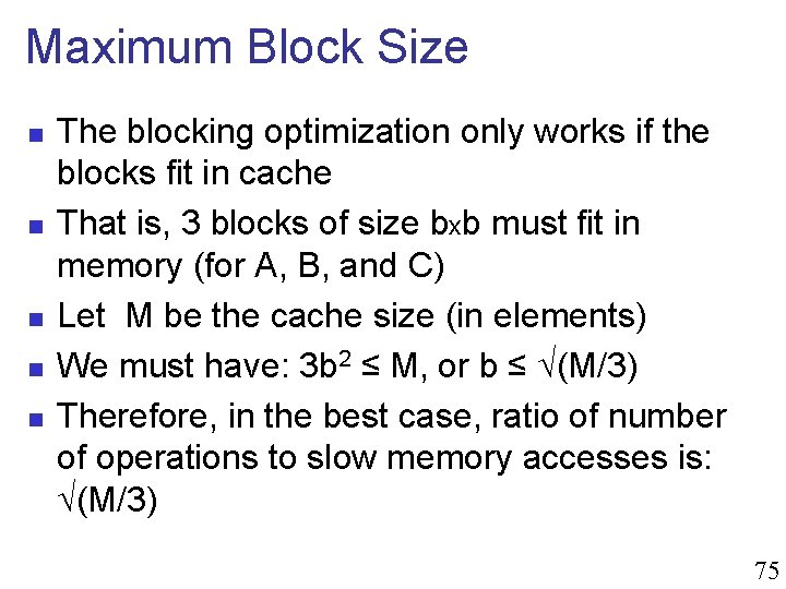
Maximum Block Size n n n The blocking optimization only works if the blocks fit in cache That is, 3 blocks of size bxb must fit in memory (for A, B, and C) Let M be the cache size (in elements) We must have: 3 b 2 ≤ M, or b ≤ √(M/3) Therefore, in the best case, ratio of number of operations to slow memory accesses is: √(M/3) 75

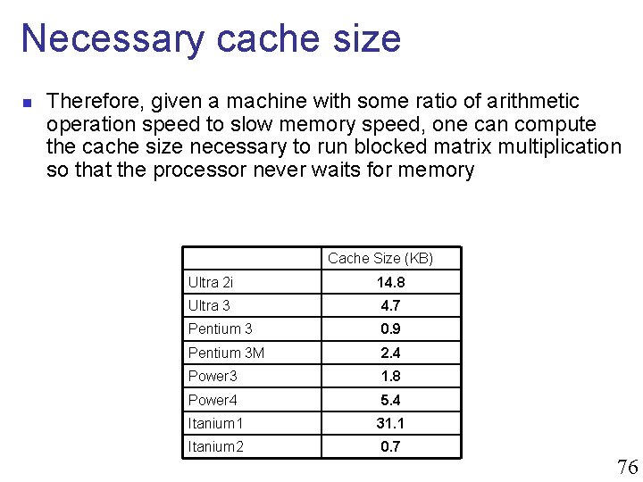
Necessary cache size n Therefore, given a machine with some ratio of arithmetic operation speed to slow memory speed, one can compute the cache size necessary to run blocked matrix multiplication so that the processor never waits for memory Cache Size (KB) Ultra 2 i 14. 8 Ultra 3 4. 7 Pentium 3 0. 9 Pentium 3 M 2. 4 Power 3 1. 8 Power 4 5. 4 Itanium 1 31. 1 Itanium 2 0. 7 76

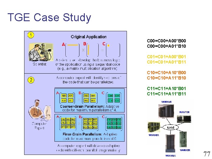
TGE Case Study C 00=C 00+A 00*B 00 C 00=C 00+A 01*B 10 C 01=C 01+A 00*B 01 C 01=C 01+A 01*B 11 C 10=C 10+A 10*B 00 C 10=C 10+A 11*B 10 C 11=C 11+A 10*B 01 C 11=C 11+A 11*B 11 77

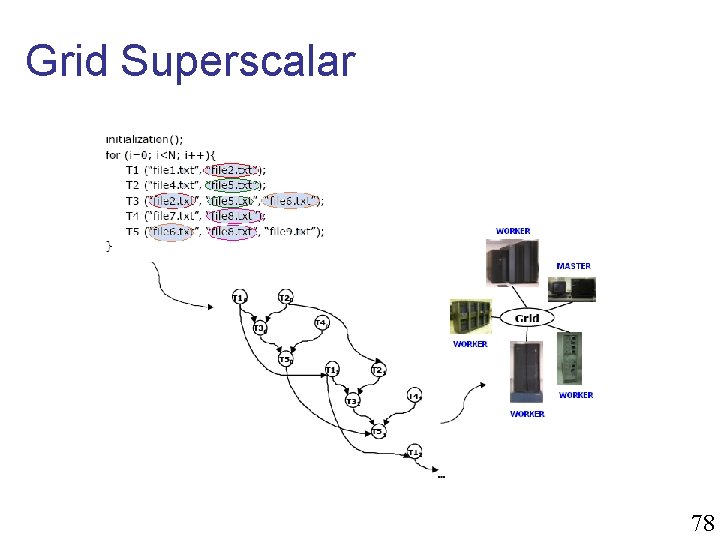
Grid Superscalar 78

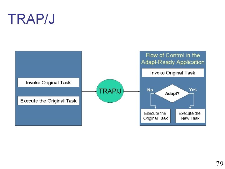
TRAP/J 79

Integration 1. 2. 3. 4. 5. We start with the original Sequential Code. Grid Superscalar – Stubs and Skeletons TRAP/J – Delegate and Wrapper class Compilation and binding of Delegate and Original Application Grid Enabled Application is obtained! 80

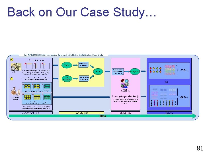
Back on Our Case Study… 81

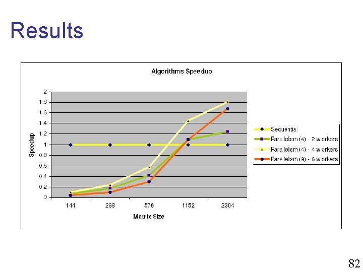
Results 82

Strassen’s Matrix Multiplication n n The traditional algorithm (w/ or w/o blocking) has O(n^3) flops Strassen discovered an algorithm with asymptotically lower flops n n O(n^2. 81) Consider a 2 x 2 matrix multiply n n Normally it takes 8 multiplies, 7 adds Strassen does it with 7 multiplies and 18 adds, which is faster! Let M = m 11 m 12 = a 11 a 12 b 11 b 12 m 21 m 22 = a 21 a 22 b 21 b 22 Let p 1 = (a 12 - a 22) * (b 21 + b 22) p 5 = a 11 * (b 12 - b 22) p 2 = (a 11 + a 22) * (b 11 + b 22) p 6 = a 22 * (b 21 - b 11) p 3 = (a 11 - a 21) * (b 11 + b 12) p 7 = (a 21 + a 22) * b 11 p 4 = (a 11 + a 12) * b 22 Then m 11 = p 1 + p 2 - p 4 + p 6 m 12 = p 4 + p 5 Extends to nxn by divide&conquer m 21 = p 6 + p 7 m 22 = p 2 - p 3 + p 5 - p 7 83

Overall Lessons n n Truly understanding application/cache behavior is tricky But approximations can be obtained by which one can reason about how to improve an implementation The notion of blocking is a common recurrence in many algorithms and applications You’ll write a blocked matrix multiplication in a Programming Assignment n not hard, but tricky with indices and loops 84

Automatic Program Generation n It is difficult to optimize code because n n n There are many possible options for tuning/modifying the code These options interact in complex ways with the compiler and the hardware This is really an “optimization problem” n n The objective function is the code’s performance The feasible solutions are all possible ways to implement the software Typically a finite number of implementation decisions are to be made Each decision can take a range of values n n e. g. , the 7 th loop in the 3 rd function can be unrolled 1, 2, . . . , 20 times e. g. , the “block size” could be 2 x 2, 4 x 4, . . . , 400 x 400 e. g. , function could be recursive or iterative And one needs to do it again and again for different platforms 85

Automatic Program Generation n What is good at solving hard optimization problems? n n computers Therefore, a computer program could generate the computer program with the best performance n Could use a brute force approach: try all possible solutions n n n but there is an exponential number of them Could use genetic algorithms Could use some ad-hoc optimization technique 86

Matrix Multiplication n We have seen that for matrix multiplication there are several possible ways to optimize the code n n n block size optimization flag to the compiler order of loops. . . It is difficult to find the best one People have written automatic matrix multiplication program generators! 87

The ATLAS Project n n n ATLAS is a software that you can download and run on most platforms. It runs for a while (perhaps a couple of hours) and generates a. c file that implements matrix multiplication! ATLAS optimizes for n n Instruction cache reuse Floating point instruction ordering n n n Reducing loop overhead Exposing parallelism n n pipeline functional units multiple functional units Cache reuse 88

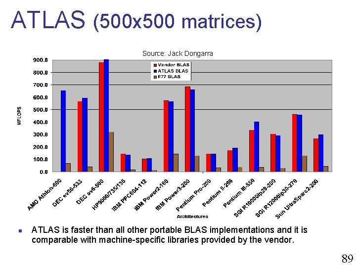
ATLAS (500 x 500 matrices) Source: Jack Dongarra n ATLAS is faster than all other portable BLAS implementations and it is comparable with machine-specific libraries provided by the vendor. 89

Conclusions n Programming for performance means working with the compiler n n knowing its limitations knowing its capabilities if it is unhindered Finding the optimal code is really difficult, but dealing with locality is paramount Automatic approaches for generating the code have been very successful in some cases 90