Hand in your Homework Assignment Introduction to Statistics

Hand in your Homework Assignment

Introduction to Statistics for the Social Sciences SBS 200 - Lecture Section 001, Fall 2017 Room 150 Harvill Building 10: 00 - 10: 50 Mondays, Wednesdays & Fridays.

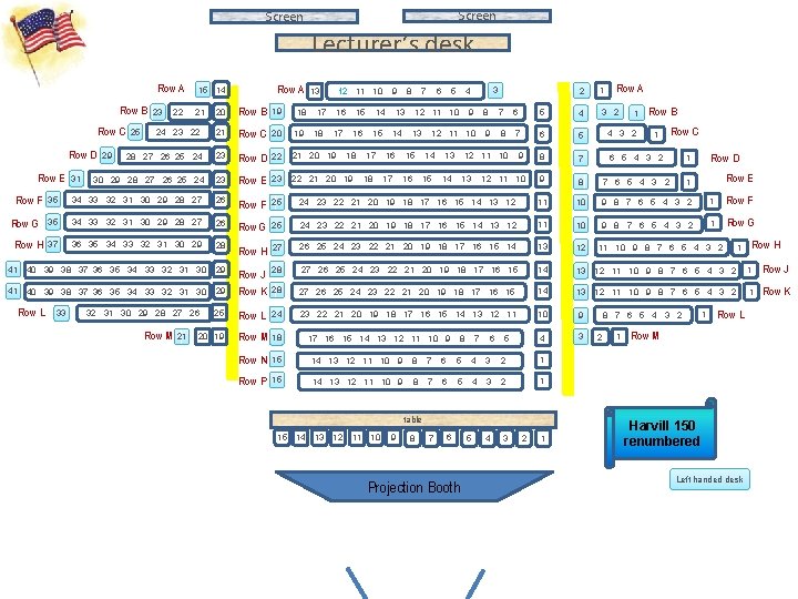
Screen Lecturer’s desk Row A Row B Row A 15 14 12 11 10 13 20 Row B 19 24 23 22 21 Row C 20 19 28 27 26 25 24 23 Row D 22 21 20 19 30 29 28 27 26 25 24 23 Row E 23 22 21 20 19 35 34 33 32 31 30 29 28 27 26 Row F 25 35 34 33 32 31 30 29 28 27 26 Row G 37 36 35 34 33 32 31 30 29 28 41 40 39 38 37 36 35 34 33 32 31 30 Row C Row D Row E Row F Row G Row H Row L 33 31 29 25 23 22 21 21 8 7 6 5 3 4 Row A 2 1 3 2 Row B 9 8 7 6 5 4 12 11 10 9 8 7 6 5 4 3 2 1 24 23 22 21 20 19 18 17 16 15 14 13 12 11 10 9 8 7 6 5 4 3 2 1 Row F 25 24 23 22 21 20 19 18 17 16 15 14 13 12 11 10 9 8 7 6 5 4 3 2 1 Row G Row H 27 26 25 24 23 22 21 20 19 18 17 16 15 14 13 12 29 Row J 28 27 26 25 24 23 22 21 20 19 18 17 16 15 14 13 12 11 10 9 8 7 6 5 4 3 2 1 Row J 29 Row K 28 27 26 25 24 23 22 21 20 19 18 17 16 15 14 13 12 11 10 9 8 7 6 5 4 3 2 1 Row K 25 Row L 24 23 22 21 20 19 18 17 16 15 14 13 12 11 10 9 20 19 Row M 18 4 3 Row N 15 14 13 12 11 10 9 8 7 6 5 4 3 2 1 Row P 15 14 13 12 11 10 9 8 7 6 5 4 3 2 1 4 3 32 31 30 29 28 27 26 Row M 9 18 17 18 16 17 15 16 18 14 15 17 18 13 14 13 16 17 12 11 10 15 16 14 15 13 12 11 10 14 17 16 15 14 13 12 11 10 9 13 8 7 6 5 table 15 14 13 12 11 10 9 8 7 6 Projection Booth 5 2 1 1 1 Row C Row D Row E 11 10 9 8 7 6 5 4 3 2 2 1 1 1 Row L Row M Harvill 150 renumbered Left handed desk Row H

A note on doodling

Everyone will want to be enrolled in one of the lab sessions Labs all done with Presentations Start Project 3 Next Week

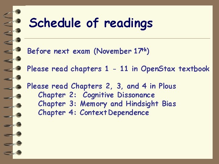
Schedule of readings Before next exam (November 17 th) Please read chapters 1 - 11 in Open. Stax textbook Please read Chapters 2, 3, and 4 in Plous Chapter 2: Cognitive Dissonance Chapter 3: Memory and Hindsight Bias Chapter 4: Context Dependence

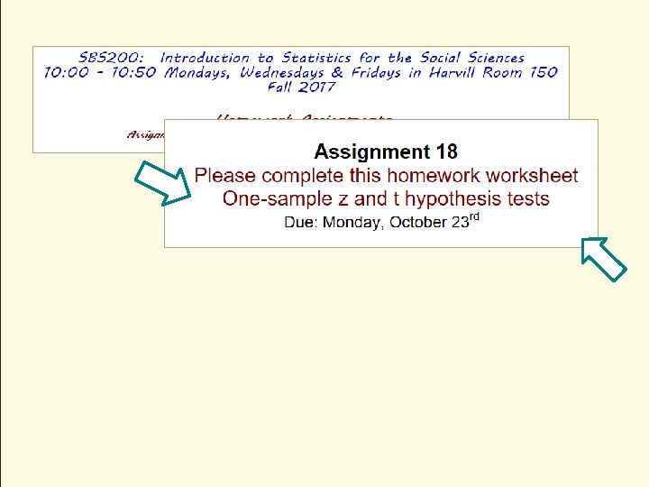
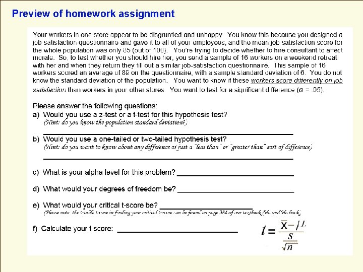
Preview of homework assignment

Preview of homework assignment

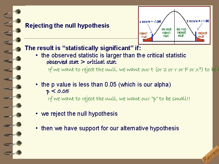
Rejecting the null hypothesis The result is “statistically significant” if: • the observed statistic is larger than the critical statistic observed stat > critical stat If we want to reject the null, we want our t (or z or r or F or x 2) to be b • the p value is less than 0. 05 (which is our alpha) p < 0. 05 If we want to reject the null, we want our “p” to be small!! • we reject the null hypothesis • then we have support for our alternative hypothesis Re w e i v

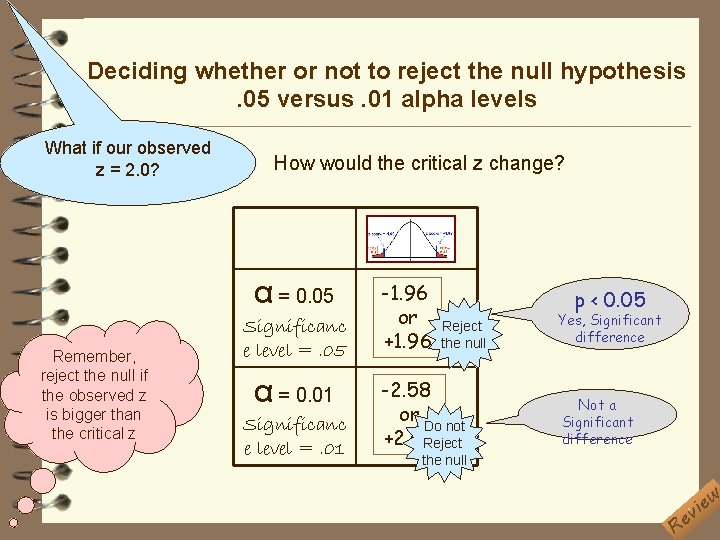
Deciding whether or not to reject the null hypothesis. 05 versus. 01 alpha levels What if our observed z = 2. 0? How would the critical z change? α = 0. 05 Remember, reject the null if the observed z is bigger than the critical z Significanc e level =. 05 α = 0. 01 Significanc e level =. 01 -1. 96 or +1. 96 p < 0. 05 Reject the null -2. 58 or Do not +2. 58 Reject Yes, Significant difference Not a Significant difference the null Re w e i v

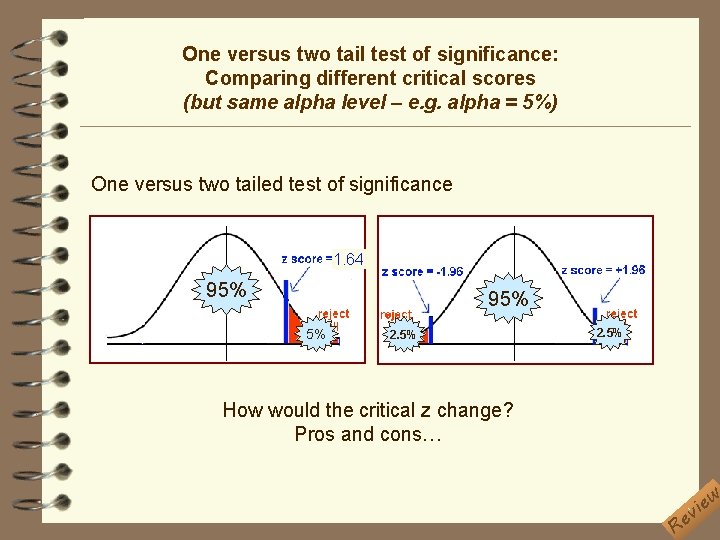
One versus two tail test of significance: Comparing different critical scores (but same alpha level – e. g. alpha = 5%) One versus two tailed test of significance 1. 64 95% 5% 2. 5% How would the critical z change? Pros and cons… Re w e i v

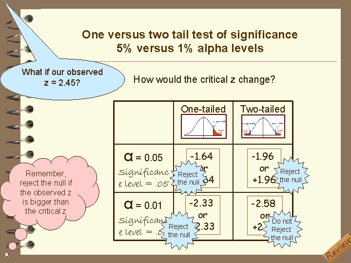
One versus two tail test of significance 5% versus 1% alpha levels What if our observed z = 2. 45? How would the critical z change? One-tailed α = 0. 05 Remember, reject the null if the observed z is bigger than the critical z -1. 64 Significanc Reject or +1. 64 e level =. 05 the null α = 0. 01 -2. 33 or Significanc Reject +2. 33 e level =. 01 the null Two-tailed -1. 96 or +1. 96 Reject the null -2. 58 or Do not +2. 58 Reject the null Re w e i v

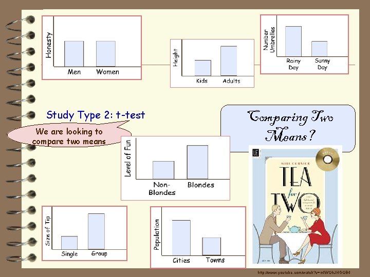
Study Type 2: t-test We are looking to compare two means Comparing Two Means? Use a t-test http: //www. youtube. com/watch? v=n 4 WQh. JHGQB 4

Study Type 2: t-test We are looking to compare two means Comparing Two Means? Use a t-test http: //www. youtube. com/watch? v=n 4 WQh. JHGQB 4

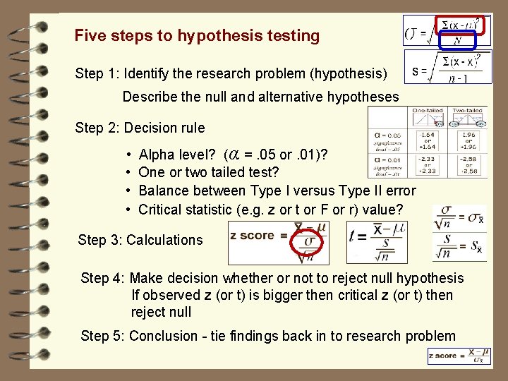
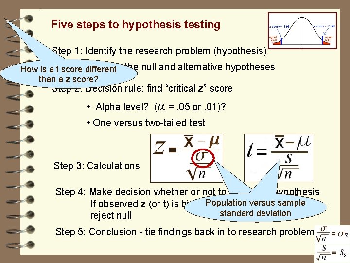
Five steps to hypothesis testing Step 1: Identify the research problem (hypothesis) Describe the null and alternative hypotheses Step 2: Decision rule • • Alpha level? (α =. 05 or. 01)? One or two tailed test? Balance between Type I versus Type II error Critical statistic (e. g. z or t or F or r) value? Step 3: Calculations Step 4: Make decision whether or not to reject null hypothesis If observed z (or t) is bigger then critical z (or t) then reject null Step 5: Conclusion - tie findings back in to research problem

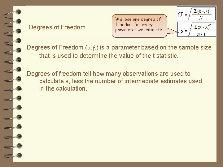
Degrees of Freedom We lose one degree of freedom for every parameter we estimate Degrees of Freedom (d. f. ) is a parameter based on the sample size that is used to determine the value of the t statistic. Degrees of freedom tell how many observations are used to calculate s, less the number of intermediate estimates used in the calculation.

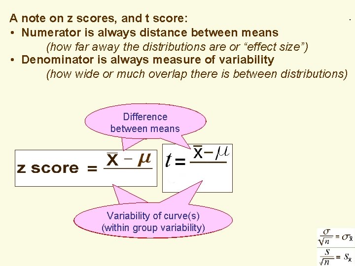
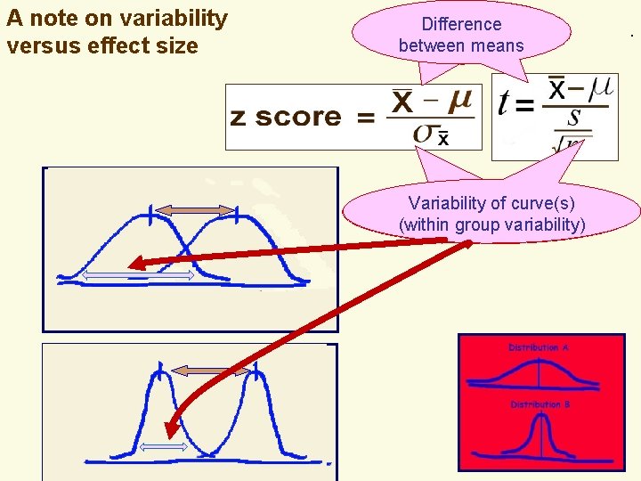
. . A note on z scores, and t score: • Numerator is always distance between means (how far away the distributions are or “effect size”) • Denominator is always measure of variability (how wide or much overlap there is between distributions) Difference between means Variability of curve(s) Variability (withinof group variability) curve(s)

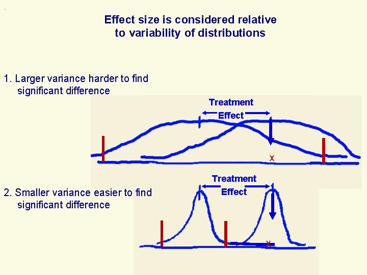
. Effect size is considered relative to variability of distributions 1. Larger variance harder to find significant difference Treatment Effect x 2. Smaller variance easier to find significant difference Treatment Effect x

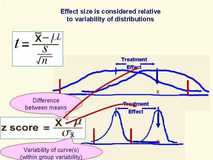
. Effect size is considered relative to variability of distributions Treatment Effect x Difference between means Treatment Effect x Variability of curve(s) (within group variability)

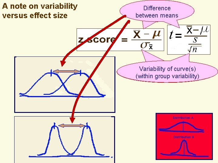
. A note on variability versus effect size Difference between means Variability of curve(s) Variability (withinof group variability) curve(s)

. A note on variability versus effect size Difference between means Variability of curve(s) Variability (withinof group variability) curve(s) .

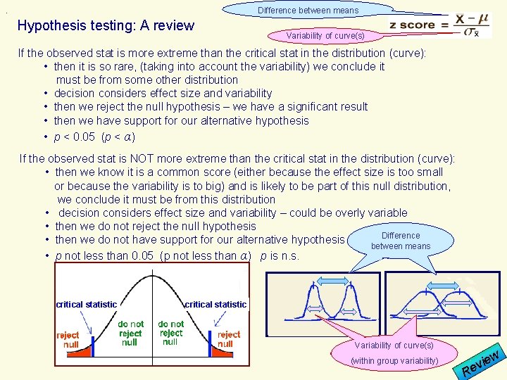
. Difference between means Hypothesis testing: A review Variability of curve(s) If the observed stat is more extreme than the critical stat in the distribution (curve): • then it is so rare, (taking into account the variability) we conclude it must be from some other distribution • decision considers effect size and variability • then we reject the null hypothesis – we have a significant result • then we have support for our alternative hypothesis • p < 0. 05 (p < α) If the observed stat is NOT more extreme than the critical stat in the distribution (curve): • then we know it is a common score (either because the effect size is too small or because the variability is to big) and is likely to be part of this null distribution, we conclude it must be from this distribution • decision considers effect size and variability – could be overly variable • then we do not reject the null hypothesis Difference • then we do not have support for our alternative hypothesis between means • p not less than 0. 05 (p not less than α) p is n. s. critical statistic Variability of curve(s) (within group variability) iew v Re

Five steps to hypothesis testing Step 1: Identify the research problem (hypothesis) How is a t score Describe different the null and alternative hypotheses than a z score? Step 2: Decision rule: find “critical z” score • Alpha level? (α =. 05 or. 01)? • One versus two-tailed test Step 3: Calculations Step 4: Make decision whether or not to reject null hypothesis versus sample If observed z (or t) is bigger. Population then critical z (or t) then standard deviation reject null Step 5: Conclusion - tie findings back in to research problem

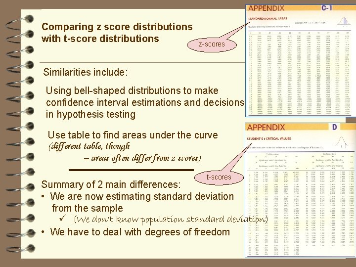
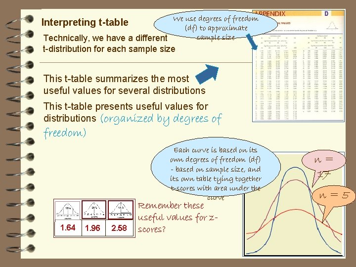
Comparing z score distributions with t-score distributions z-scores Similarities include: Using bell-shaped distributions to make confidence interval estimations and decisions in hypothesis testing Use table to find areas under the curve (different table, though – areas often differ from z scores) t-scores Summary of 2 main differences: • We are now estimating standard deviation from the sample ü (We don’t know population standard deviation) • We have to deal with degrees of freedom

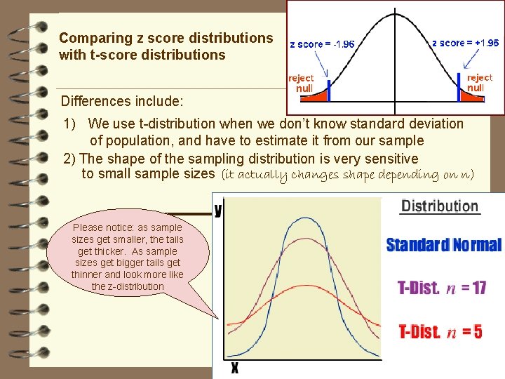
Comparing z score distributions with t-score distributions Differences include: 1) We use t-distribution when we don’t know standard deviation of population, and have to estimate it from our sample 2) The shape of the sampling distribution is very sensitive to small sample sizes (it actually changes shape depending on n) Please notice: as sample sizes get smaller, the tails get thicker. As sample sizes get bigger tails get thinner and look more like the z-distribution

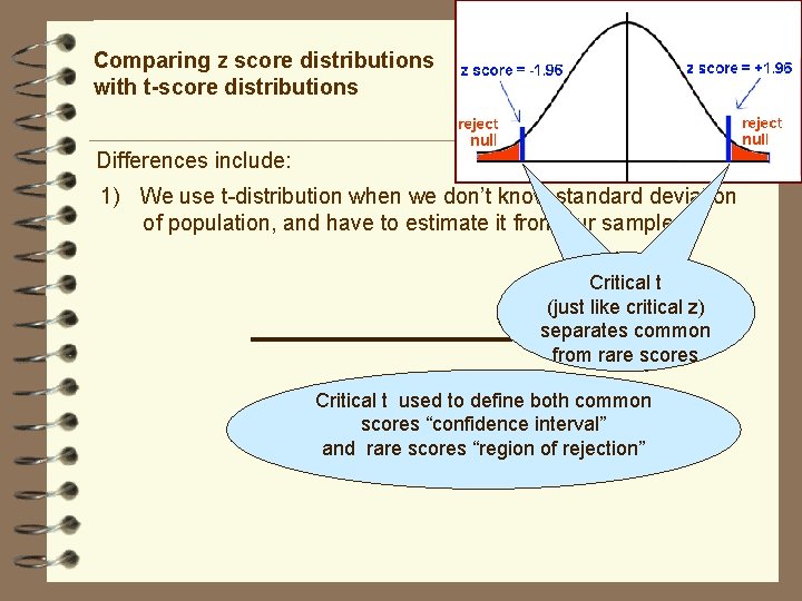
Comparing z score distributions with t-score distributions Differences include: 1) We use t-distribution when we don’t know standard deviation of population, and have to estimate it from our sample Critical t (just like critical z) separates common from rare scores Critical t used to define both common scores “confidence interval” and rare scores “region of rejection”

Comparing z score distributions with t-score distributions Differences include: 1) We use t-distribution when we don’t know standard deviation of population, and have to estimate it from our sample 2) The shape of the sampling distribution is very sensitive to small sample sizes (it actually changes shape depending on n) Please notice: as sample sizes get smaller, the tails get thicker. As sample sizes get bigger tails get thinner and look more like the z-distribution

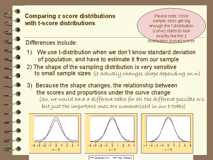
Comparing z score distributions with t-score distributions Differences include: Please note: Once sample sizes get big enough the t distribution (curve) starts to look exactly like the z distribution (curve) scores 1) We use t-distribution when we don’t know standard deviation of population, and have to estimate it from our sample 2) The shape of the sampling distribution is very sensitive to small sample sizes (it actually changes shape depending on n) 3) Because the shape changes, the relationship between the scores and proportions under the curve change (So, we would have a different table for all the different possible n’s but just the important ones are summarized in our t-table)

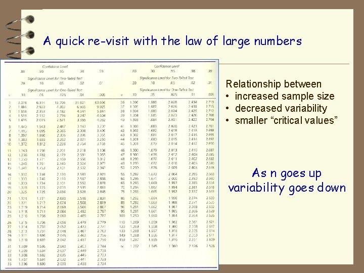
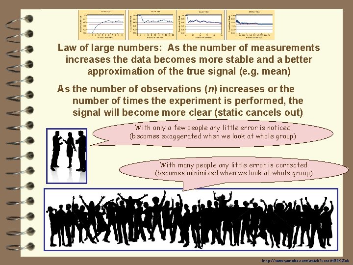
A quick re-visit with the law of large numbers Relationship between • increased sample size • decreased variability • smaller “critical values” As n goes up variability goes down

Law of large numbers: As the number of measurements increases the data becomes more stable and a better approximation of the true signal (e. g. mean) As the number of observations (n) increases or the number of times the experiment is performed, the signal will become more clear (static cancels out) With only a few people any little error is noticed (becomes exaggerated when we look at whole group) With many people any little error is corrected (becomes minimized when we look at whole group) http: //www. youtube. com/watch? v=ne 6 t. B 2 Ki. Zuk

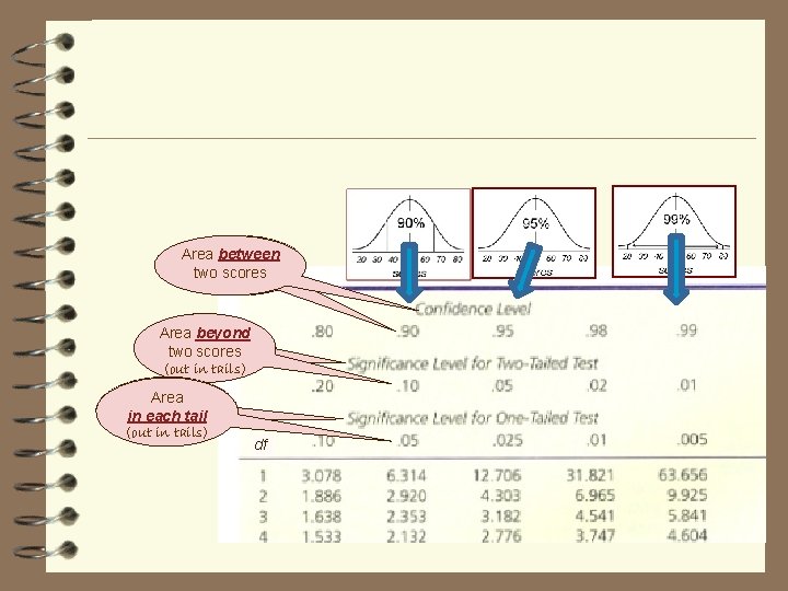
We use degrees of freedom (df) to approximate sample size Technically, we have a different Interpreting t-table t-distribution for each sample size This t-table summarizes the most useful values for several distributions This t-table presents useful values for distributions (organized by degrees freedom) Each curve is based on its own degrees of freedom (df) - based on sample size, and its own table tying together t-scores with area under the curve . 1. 64 1. 96 of 2. 58 Remember these useful values for zscores? n= 17 n=5

Areabetween two twoscores Area beyond two scores (out in tails) Area in each tail (out in tails) df

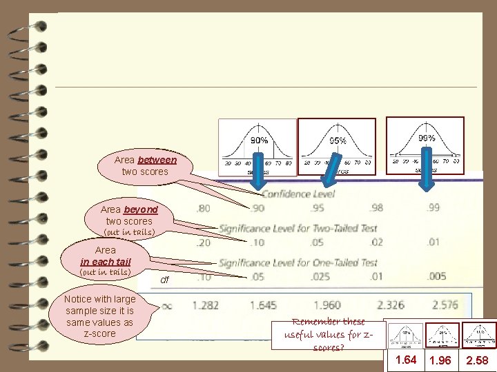
Areabetween two twoscores Area beyond two scores (out in tails) Area in each tail (out in tails) Notice with large sample size it is same values as z-score df Remember these useful values for zscores? . 1. 64 1. 96 2. 58

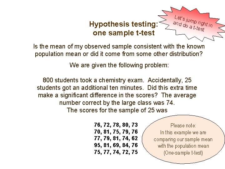
Hypothesis testing: one sample t-test Let’s ju and d mp right i n o a ttest Is the mean of my observed sample consistent with the known population mean or did it come from some other distribution? We are given the following problem: 800 students took a chemistry exam. Accidentally, 25 students got an additional ten minutes. Did this extra time make a significant difference in the scores? The average number correct by the large class was 74. The scores for the sample of 25 was 76, 72, 78, 80, 73 70, 81, 75, 79, 76 77, 79, 81, 74, 62 95, 81, 69, 84, 76 75, 77, 74, 72, 75 Please note: In this example we are comparing our sample mean with the population mean (One-sample t-test)

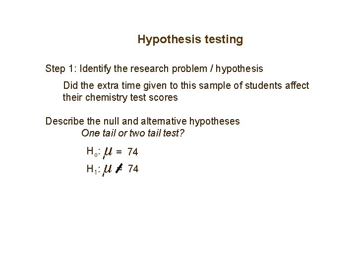
Hypothesis testing Step 1: Identify the research problem / hypothesis Did the extra time given to this sample of students affect their chemistry test scores Describe the null and alternative hypotheses One tail or two tail test? µ = 74 H : µ = 74 Ho : 1

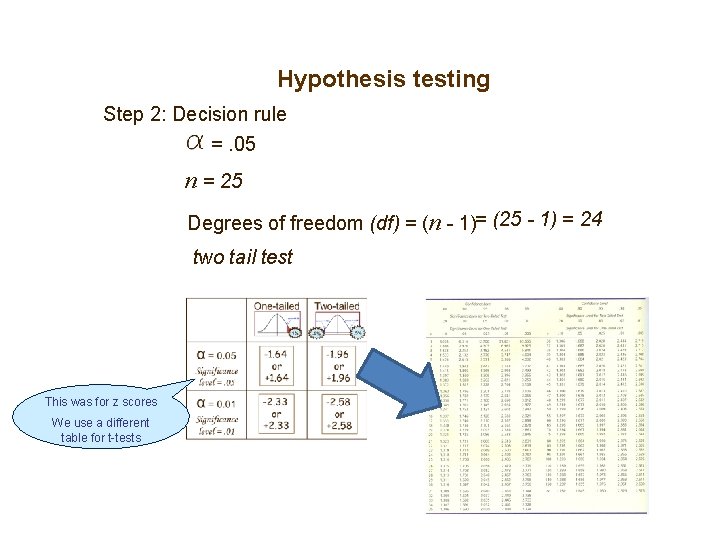
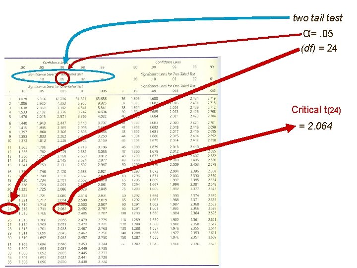
Hypothesis testing Step 2: Decision rule =. 05 n = 25 Degrees of freedom (df) = (n - 1)= (25 - 1) = 24 two tail test This was for z scores We use a different table for t-tests

two tail test α=. 05 (df) = 24 Critical t(24) = 2. 064

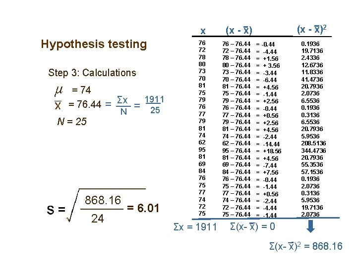
Hypothesis testing Step 3: Calculations µ = 74 = 76. 44 N = 25 = Σx = N 868. 16 24 1911 25 = 6. 01 x (x - x) 76 72 78 80 73 70 81 75 79 76 77 79 81 74 62 95 81 69 84 76 75 77 74 72 75 76 – 76. 44 72 – 76. 44 78 – 76. 44 80 – 76. 44 73 – 76. 44 70 – 76. 44 81 – 76. 44 75 – 76. 44 79 – 76. 44 76 – 76. 44 77 – 76. 44 79 – 76. 44 81 – 76. 44 74 – 76. 44 62 – 76. 44 95 – 76. 44 81 – 76. 44 69 – 76. 44 84 – 76. 44 76 – 76. 44 75 – 76. 44 77 – 76. 44 74 – 76. 44 72 – 76. 44 75 – 76. 44 Σx = 1911 (x - x)2 = -0. 44 = -4. 44 = +1. 56 = + 3. 56 = -3. 44 = -6. 44 = +4. 56 = -1. 44 = +2. 56 = -0. 44 = +0. 56 = +2. 56 = +4. 56 = -2. 44 = -14. 44 = +18. 56 = +4. 56 = -7. 44 = +7. 56 = -0. 44 = -1. 44 = +0. 56 = -2. 44 = -4. 44 = -1. 44 0. 1936 19. 7136 2. 4336 12. 6736 11. 8336 41. 4736 20. 7936 2. 0736 6. 5536 0. 1936 0. 3136 6. 5536 20. 7936 5. 9536 208. 5136 344. 4736 20. 7936 55. 3536 57. 1536 0. 1936 2. 0736 0. 3136 5. 9536 19. 7136 2. 0736 Σ(x- x) = 0 Σ(x- x)2 = 868. 16

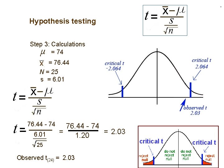
. Hypothesis testing Step 3: Calculations = 74 µ = 76. 44 N = 25 s = 6. 01 76. 44 - 74 = = 2. 03 1. 20 25 Observed t(24) = 2. 03 critical t

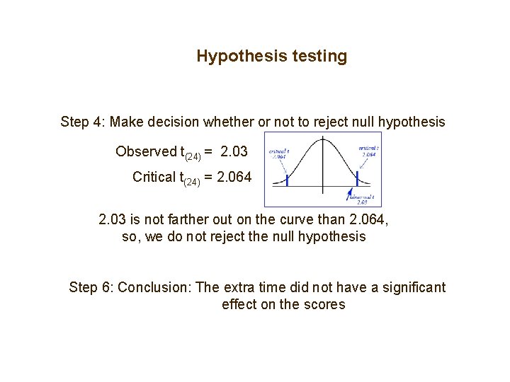
Hypothesis testing Step 4: Make decision whether or not to reject null hypothesis Observed t(24) = 2. 03 Critical t(24) = 2. 064 2. 03 is not farther out on the curve than 2. 064, so, we do not reject the null hypothesis Step 6: Conclusion: The extra time did not have a significant effect on the scores

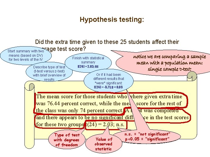
Hypothesis testing: Did the extra time given to these 25 students affect their average test score? Start summary with two means (based on DV) for two levels of the IV Describe type of test (t-test versus z-test) with brief overview of results Finish with statistical summary t(24) = 2. 03; ns notice we are comparing a sample mean with a population mean: single sample t-test Or if it had been different results that *were* significant: t(24) = -5. 71; p < 0. 05 The mean score for those students who where given extra time was 76. 44 percent correct, while the mean score for the rest of the class was only 74 percent correct. A t-test was completed and there appears to be no significant difference in the test scores for these two groups t(24) = 2. 03; n. s. Type of test with degrees of freedom Value of observed statistic n. s. = “not significant” p<0. 05 = “significant”