Giovanni Succi 21042020 Outline Introduction Mathematical description of

Giovanni Succi – 21/04/2020

Outline Ø Introduction Ø Mathematical description of the problem Ø The Model Ø Case studies: Constant cable current and Ramp-up Ø Network breakdown mechanism Ø Characteristic times and lengths of the system Ø Comparison with experimental tests (at SM 18) Ø Some other considerations Ø Conclusions

Introduction • Current distribution and redistribution phenomena in multi-strand superconducting cables have been studied for over 40 years, due to their impact on field quality and stability margin of accelerator magnets. • The aim is to evaluate the effect of strand breakages, originated for instance, during the fabrication stages of coils and magnets, on the operational margin of the magnets themselves. Such an evaluation is relevant to determine if potentially damaged coils could still be employed for the magnets of the High-Luminosity project.

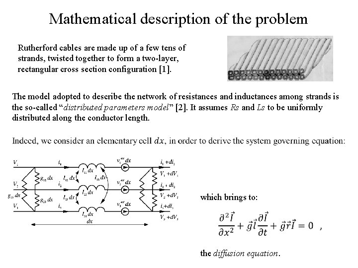
Mathematical description of the problem Rutherford cables are made up of a few tens of strands, twisted together to form a two-layer, rectangular cross section configuration [1]. The model adopted to describe the network of resistances and inductances among strands is the so-called “distributed parameters model” [2]. It assumes Rs and Ls to be uniformly distributed along the conductor length. which brings to: the diffusion equation.

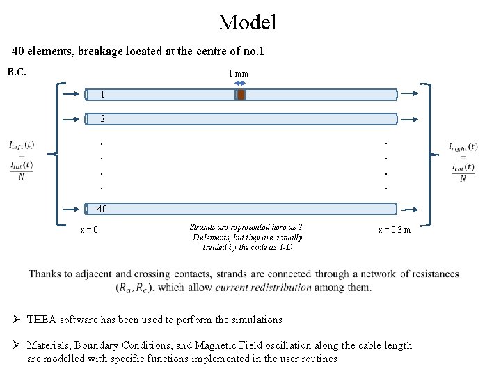
Model 40 elements, breakage located at the centre of no. 1 B. C. 1 mm 1 2 . . . . 40 x=0 Strands are represented here as 2 D elements, but they are actually treated by the code as 1 -D x = 0. 3 m Ø THEA software has been used to perform the simulations Ø Materials, Boundary Conditions, and Magnetic Field oscillation along the cable length are modelled with specific functions implemented in the user routines

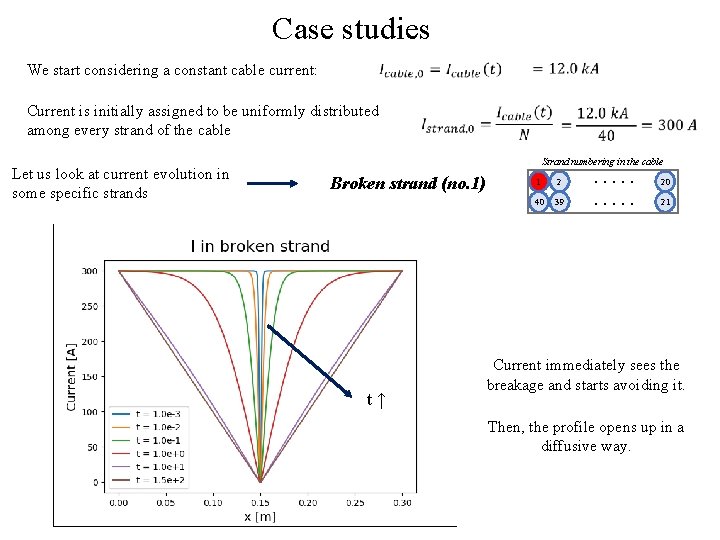
Case studies We start considering a constant cable current: Current is initially assigned to be uniformly distributed among every strand of the cable Let us look at current evolution in some specific strands Strand numbering in the cable Broken strand (no. 1) t↑ 1 2 40 39 . . 20 21 Current immediately sees the breakage and starts avoiding it. Then, the profile opens up in a diffusive way.

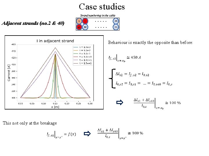
Case studies Strand numbering in the cable Adjacent strands (no. 2 & 40) 1 2 40 39 . . 20 21 Behaviour is exactly the opposite than before: This not only at the breakage

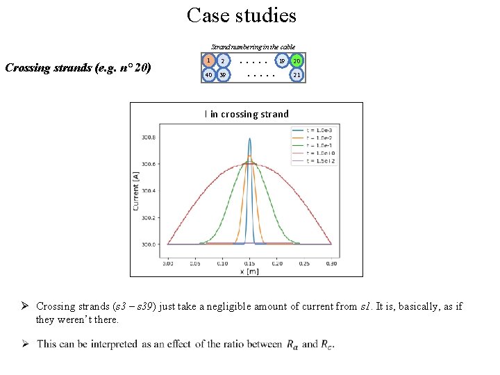
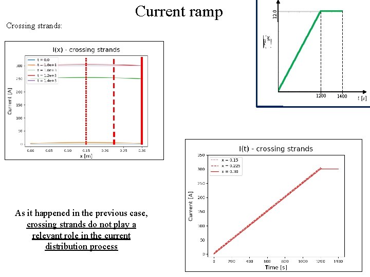
Case studies Strand numbering in the cable Crossing strands (e. g. n° 20) 1 2 40 39 . . . 19. . . 20 21 I in crossing strand Ø Crossing strands (s 3 – s 39) just take a negligible amount of current from s 1. It is, basically, as if they weren’t there.

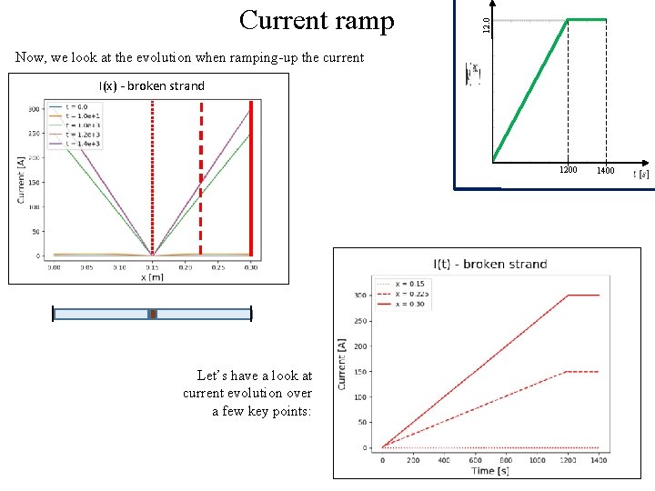
12. 0 Current ramp Now, we look at the evolution when ramping-up the current I(x) - broken strand 1200 Let’s have a look at current evolution over a few key points: 1400

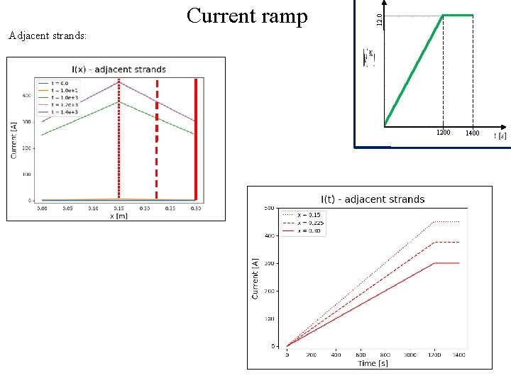
12. 0 Current ramp Adjacent strands: 1200 1400

12. 0 Current ramp Crossing strands: 1200 As it happened in the previous case, crossing strands do not play a relevant role in the current distribution process 1400

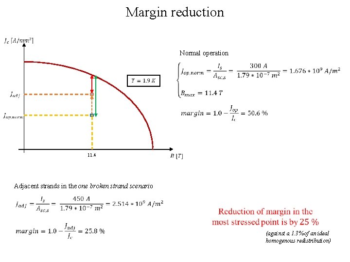
Margin reduction Normal operation 11. 4 Adjacent strands in the one broken strand scenario (against a 1. 3% of an ideal homogenous redistribution)

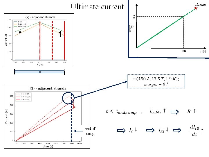
Ultimate current 12. 0 ultimate 1200 end of ramp

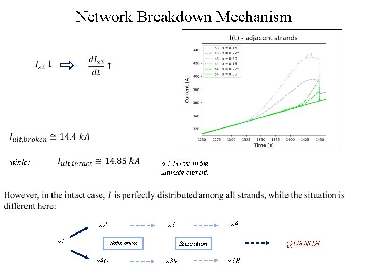
Network Breakdown Mechanism while: a 3 % loss in the ultimate current. s 2 s 1 Saturation s 40 s 4 s 3 QUENCH Saturation s 39 s 38

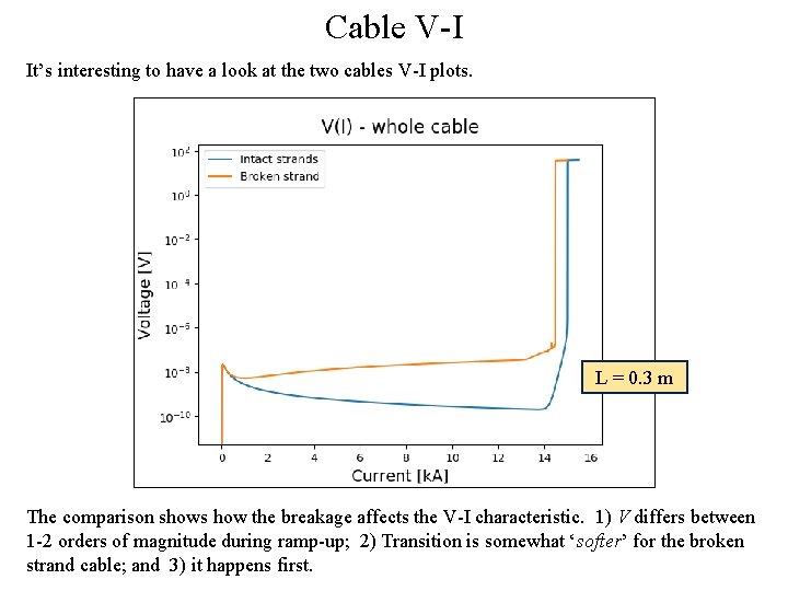
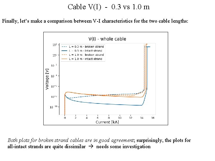
Cable V-I It’s interesting to have a look at the two cables V-I plots. L = 0. 3 m The comparison shows how the breakage affects the V-I characteristic. 1) V differs between 1 -2 orders of magnitude during ramp-up; 2) Transition is somewhat ‘softer’ for the broken strand cable; and 3) it happens first.

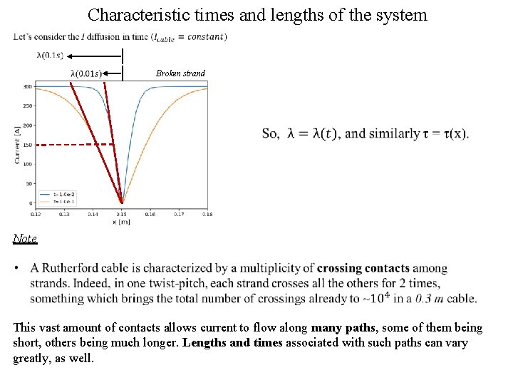
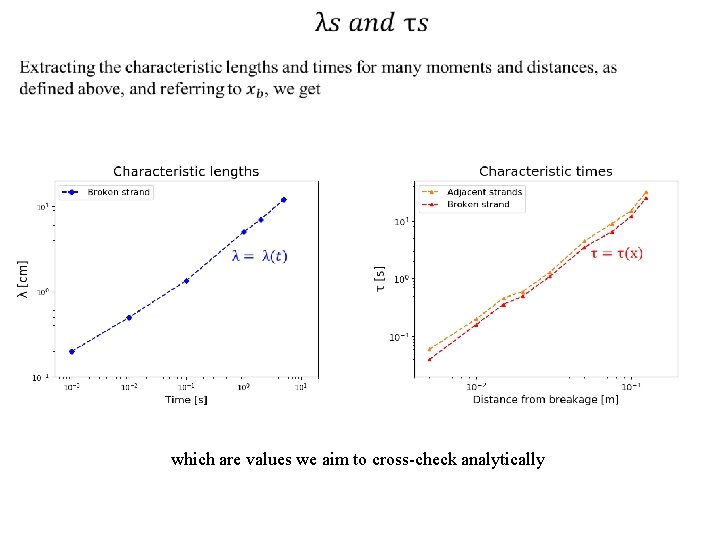
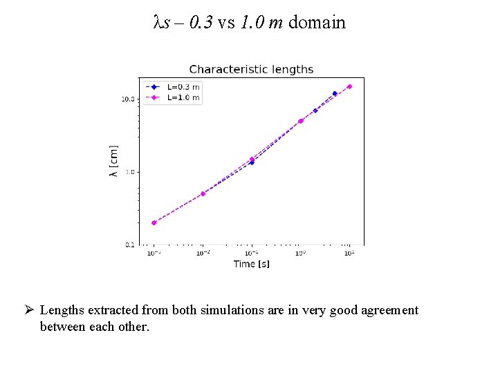
Characteristic times and lengths of the system Broken strand Note This vast amount of contacts allows current to flow along many paths, some of them being short, others being much longer. Lengths and times associated with such paths can vary greatly, as well.

which are values we aim to cross-check analytically

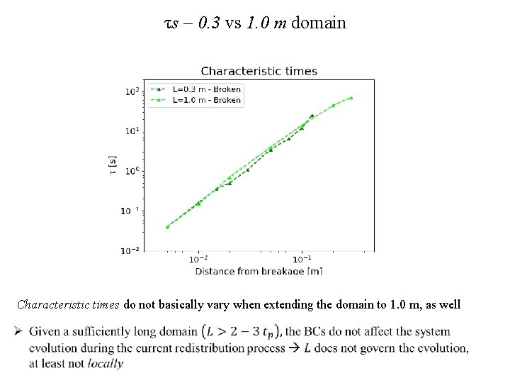
An analytical method is described in [2] to compute the time constants spectrum for an Nstrand cable. Time constants are given as: Applying the formulation, we get the spectrum of characteristic times: Ø Time constants derived analytically go from 0. 03 up to 14. 4 s. Ø Values extracted from the simulations go from 0. 04 to 12 s, in the first 10 cm from the breakage An approach based on the so-called superstrands [3] can also be followed, to derive a single “averaged” cable time constant 1 2 40 39 . . 20 Sup 2 21 Sup 1

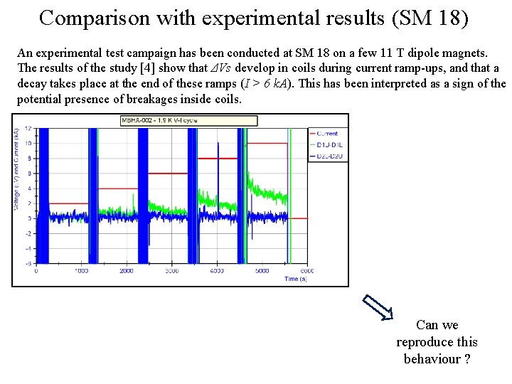
Comparison with experimental results (SM 18) An experimental test campaign has been conducted at SM 18 on a few 11 T dipole magnets. The results of the study [4] show that ΔVs develop in coils during current ramp-ups, and that a decay takes place at the end of these ramps (I > 6 k. A). This has been interpreted as a sign of the potential presence of breakages inside coils. Can we reproduce this behaviour ?

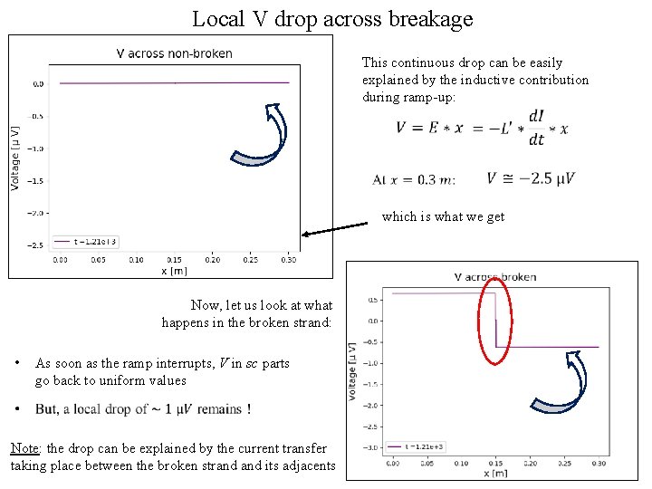
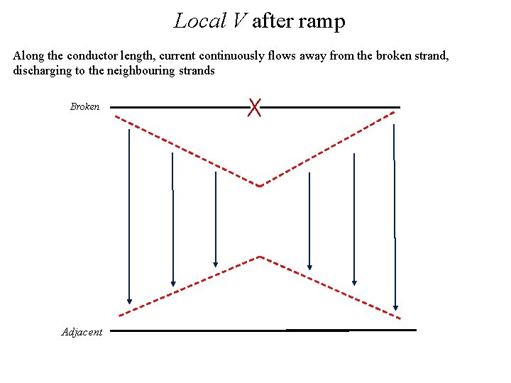
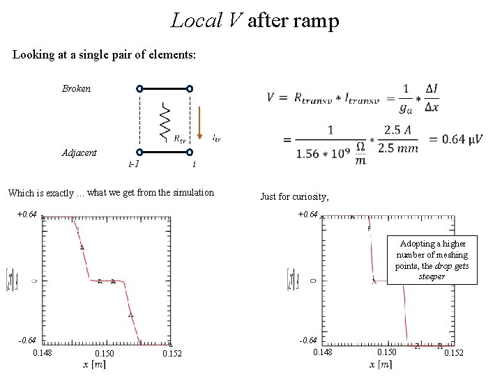
Local V drop across breakage This continuous drop can be easily explained by the inductive contribution during ramp-up: which is what we get Now, let us look at what happens in the broken strand: • As soon as the ramp interrupts, V in sc parts go back to uniform values Note: the drop can be explained by the current transfer taking place between the broken strand its adjacents Local drop development

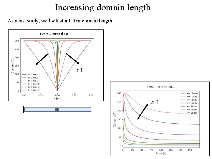
Increasing domain length As a last study, we look at a 1. 0 m domain length I vs x – strand no. 1

λs – 0. 3 vs 1. 0 m domain Ø Lengths extracted from both simulations are in very good agreement between each other.

τs – 0. 3 vs 1. 0 m domain Characteristic times do not basically vary when extending the domain to 1. 0 m, as well

Cable V(I) - 0. 3 vs 1. 0 m Finally, let’s make a comparison between V-I characteristics for the two cable lengths: Both plots for broken strand cables are in good agreement; surprisingly, the plots for all-intact strands are quite dissimilar needs some investigation

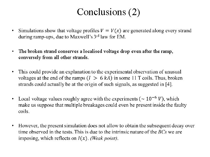
Conclusions (1) • Crossing strands do not play a relevant role in the current redistribution process. Basically, they act as “heavy ghosts”, since they just increase the total computational time. The adjacent strands, taking all the current flowing away from the broken strand, are the only ones that count.

Conclusions (2) • The broken strand conserves a localised voltage drop even after the ramp, conversely from all other strands.

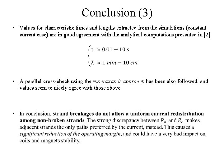
Conclusion (3) • Values for characteristic times and lengths extracted from the simulations (constant current case) are in good agreement with the analytical computations presented in [2]. • A parallel cross-check using the superstrands approach has been also followed, and values seem to nicely agree with those above.

Thanks for your attention !

Bibliography •

Back-up slides

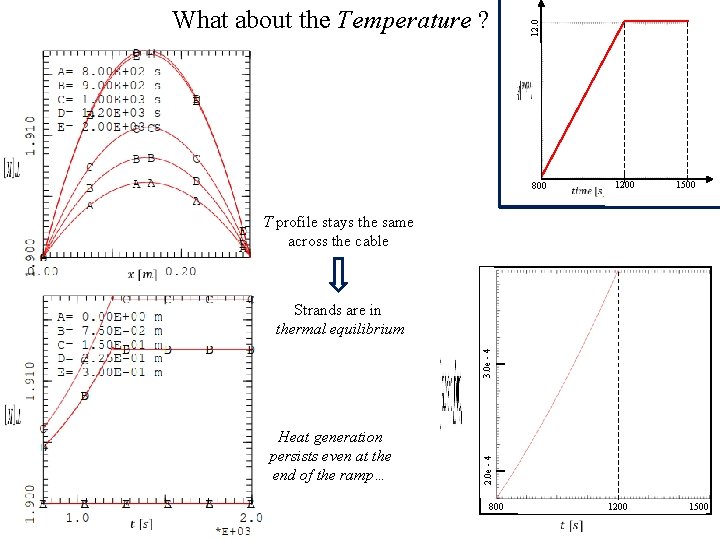
12. 0 What about the Temperature ? 800 1200 1500 T profile stays the same across the cable Heat generation persists even at the end of the ramp… 2. 0 e - 4 3. 0 e - 4 Strands are in thermal equilibrium 800 1200 1500

Local V after ramp Along the conductor length, current continuously flows away from the broken strand, discharging to the neighbouring strands Broken Adjacent

Local V after ramp Looking at a single pair of elements: Broken Adjacent i-1 i Which is exactly … what we get from the simulation +0. 64 Just for curiosity, +0. 64 Adopting a higher number of meshing points, the drop gets steeper -0. 64 0. 148 0. 150 0. 152