Finite Element Method Nonspherical cows Sauro Succi Finite

Finite Element Method (Non-spherical cows…) Sauro Succi

Finite Elements The main of FEM is to handle real-life geometries of virtually arbitrary complexity (non spherical cows) FEM achieves this task in a mathematically most elegant and systematic way. Rooted in functional analysis: very abstract but it lands down on very practical implementation strategies with the major comfort of rigorous convergence theorems.

FEM for any geometry Most powrful instance: Coordinate free (unstructured) Arbitrary shape and connectivity

FEM Theory: Functional Analysis * Hilbert space expansions * Strong vs Weak Convergence

Expansion on basis functions UNKNOWN coefficients of the expansion KNOWN set of basis functions The basis functions form a (complete) set in Hilbert space, the functional analogue of R^N vector space. Ordinary d=3 unit vectors: i=(1, 0, 0); j=(0, 1, 0), k=(0, 0, 1).

Examples basis functions Fourier: (periodic geometry) Hermite: (harmonic oscillator) Laguerre: (radial symmetry) Note that the basis functions are spatially extended

What’s the point? Convergence: By sending N to infinity ANY function in the proper Hilbert space should be approximated to arbitrary accuracy: Example: Hilbert Lp: Note that this is GLOBAL statement, less demanding than LOCAL ones: WEAK convergence

Pointwise (strong) formulation Local interpolation around x=x_j: Based on global polynomials Awkward on unstructured lattices

FEM: Practice How do we compute the unknown coeff’s? * Projetion methods Define the scalar (inner) product in Hilbert space as: Where w(x) is a suitable weight to secure finiteness Mass matrix

Co-evolutionary ODE’s Liouville equation: Hilbert-Expand: Hilbert Project: Take scalar product with each phi_1 … phi_N: CO-evolution matrix ODE’s problem: Mass matrix Liouville matrix

Co-evolutionary ODE’s Suppose the basis set is ortho-normal, i. e. Then the mass matrix is the identity and each coefficient evolves on its own: The “ray” f=(f 1, f 2 … f. N) moves in time within N-dimensional Hilberts Space spanned by phi_1 … phi_N. By making Hilbert infinite-dimensional, the exact solution is recovered. This is systematic and supported by rigorous convergence theorems. All basis functions mentioned earlier on can be made ortho-normal.

Practical concern All is well in theory, but practice often tells another story: By increasing N, orthogonality depends more and more on subtle cancellations, because the basis functions are global hence their overlap integral (mass matrix) cannot be zero unless these functions oscillate in space. This is very unhealthy from the numerical standpoint: leads to ill-fated long term solutions

FEM take stage! FEM’s are COMPACT basis functions: they are non-zero only within a finite set (whence the nomer) and strictly zero elsewhere: Piecewise linear elements (“hat functions”) Usually denoted e_j(x):

Piecewise Constant (pwc) Characteristic function Pretty low-order, not useful unless discontinuities are physical (shocks)

Piecewise Linear (pwl) Piecewise linear, C 1 class: Continuous with discontinuous derivatives Higher order (quadratic, cubic and so on) are also used, esp With PDE’s with space derivatives above second order

Expansion on local basis functions Basis function (known): Coeff’s: (UNknown):

Expansion on local basis function Projection on Hilbert space Note that the mass matrix is NOT diagonal, a price to pay to locality: the finite elements overlap with neighbors The Liouville matrix cannot be diagonal as it contains space derivatives

Finite-support basis function Note that the support extends over TWO lattice spacings (generally non uniform)

Useful identities Polynomials of order 2+ are not exactly representable by linear elements:

Variational (weak) formulation Exact: Hilbert space L 2: global statement Operational: for a sequence g_k, find f_N such that: Orthogonality in N-dim Hilbert space

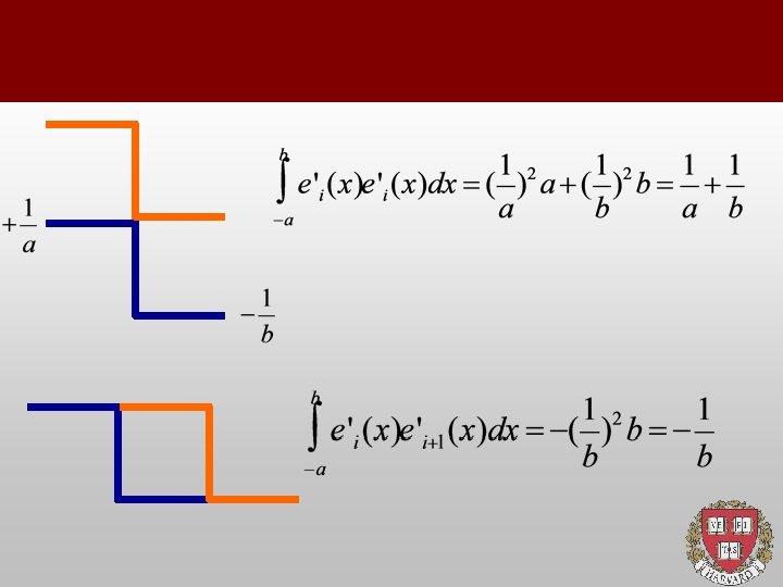
Examples of matrices: Mass, Stiffness, Advection. using linear hat functions

FEM operators

Mass matrix Algebra on the blackboard. . Uniform mesh:

Advection matrix Same as uniform mesh:

Diffusion matrix Uniform mesh:

Mass matrix: mollifier Define: F_j is a coarse-grained quantity: smoother

FEM vs FD operators

FEM code structure 1. Form the Local Matrices (Numerical Quadrature) 2. Assemble the Global Matrices (Local to Global Mapping) 3. Time Marching M*df/dt=Lf by a suitable time-marching method 4. Solve the matrix algebra problem A*f(t+dt)=B*f(t)

Matrix assembly Element-wise

Matrix assembly: 1 d 4 matrix elements per interval; 2 intervals per node= 8 matrix elements/node

Local to Global Mapping 1 2 1 In d=1 it is trivial: In d>1 a bit more laborious but still simple if the FEM are Cartesian: With unstructured meshes, no global coordinate system is available. Numbering is a task intself. More on the next lecture. 2

Time marching Index free notation: f is an array of size N: Explicit Euler: Even the explicit marching implies a matrix problem!!! (not nice) Crank-Nicolson:

Matrix Problem Index free notation: f is an array of size N: Two major families: 1. Direct Methods (Gauss Elimination) Exact (within roundoff) but expensive O(N^3). Highly sensitive to optimal numbering 2. Iterative Methods Approximate, but they involve no linear algebra other Than matrix-vector multiply, hence they take full advantage of matrix sparsity. Usually much faster, unless the matrix is very “nasty” (advection dominated). Generally recommended in d>2.

FEM for nonlinear eqs Burgers (again!) Nonlinearity brings in higher rank matrices (mode coupling) Thanks to compactness, the coupling remains local: k and l cannot be more than one spacing apart from j!

Self-advection matrix: triad Three-body coupling Uniform mesh:

Self-advection: j=k=l

Self-advection: j=k, k+1

Self-advection: j, k=j+1, l=k+1

FEM for high order PDEs Kuramoto-Sivashinsky (paradigm of chaotic PDE’s) Hat functions return ZERO: cubic elements mandatory!

Boundary Conditions 1. Periodic 2. Dirichlet 3. Neumann They are implemented at the level of the matrix and/or The right hand side, see examples

Periodic BC a 10 a. N, N+1

Dirichlet

Von-Neumann

Assignements 1. Solve the one-dimensional Poisson equation using hat FEM (Dirichlet BC) 2. Same for ADR (Periodic BC) 3. Same for Burgers

End of Lecture

Expansion on basis functions Operators to Matrices